Viscosity I: Liquid Viscosity
Michael Fowler
Introduction: Friction at the Molecular Level
Viscosity is, essentially, fluid friction. Like friction between moving solids, viscosity transforms kinetic energy of (macroscopic) motion into heat energy. Heat is energy of random motion at the molecular level, so to have any understanding of how this energy transfer takes place, it is essential to have some picture, however crude, of solids and/or liquids sliding past each other as seen on the molecular scale.
To begin with, we’ll review the molecular picture of friction between solid surfaces, and the significance of the coefficient of friction in the familiar equation Going on to fluids, we’ll give the definition of the coefficient of viscosity for liquids and gases, give some values for different fluids and temperatures, and demonstrate how the microscopic picture can give at least a qualitative understanding of how these values vary: for example, on raising the temperature, the viscosity of liquids decreases, that of gases increases. Also, the viscosity of a gas doesn’t depend in its density! These mysteries can only be unraveled at the molecular level, but there the explanations turn out to be quite simple.
As will become clear later, the coefficient of viscosity can be viewed in two rather different (but of course consistent) ways: it is a measure of how much heat is generated when faster fluid is flowing by slower fluid, but it is also a measure of the rate of transfer of momentum from the faster stream to the slower stream. Looked at in this second way, it is analogous to thermal conductivity, which is a measure of the rate of transfer of heat from a warm place to a cooler place.
Quick Review of Friction Between Solids
First, static friction: suppose a book is lying on your desk, and you tilt the desk. At a certain angle of tilt, the book begins to slide. Before that, it’s held in place by “static friction”. What does that mean on a molecular level? There must be some sort of attractive force between the book and the desk to hold the book from sliding.
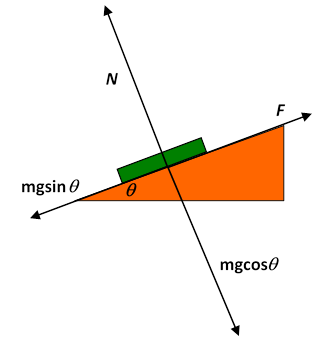
Let’s look at all the forces on the book: gravity is pulling it vertically down, and there is a “normal force” of the desk surface pushing the book in the direction normal to the desk surface. (This normal force is the springiness of the desktop, slightly compressed by the weight of the book.) When the desk is tilted, it’s best to visualize the vertical gravitational force as made up of a component normal to the surface and one parallel to the surface (downhill). The gravitational component perpendicular to the surface is exactly balanced by the normal force, and if the book is at rest, the “downhill” component of gravity is balanced by a frictional force parallel to the surface in the uphill direction. On a microscopic scale, this static frictional force is from fairly short range attractions between molecules on the desk and those of the book.
Question: but if that’s true, why does doubling the normal force double this frictional force? (Recall where is the normal force, is the limiting frictional force just before the book begins to slide, and is the coefficient of friction. By the way, the first appearance of being proportional to is in the notebooks of Leonardo da Vinci.)
Answer : Solids are almost always rough on an atomic scale: when two flat looking solid surfaces are pushed together, in fact only a tiny fraction of the common surface is really in contact at the atomic level. The stresses within that tiny area are large, the materials distort plastically and there is adhesion. The picture can be very complex, depending on the materials involved, but the bottom line is that there is only atom-atom interaction between the solids over a small area, and what happens in this small area determines the frictional force. If the normal force is doubled (by adding another book, say) the tiny area of contact between the bottom book and the desk will also doublethe true area of atomic contact increases linearly with the normal forcethat’s why friction is proportional to Within the area of “true contact” extra pressure makes little difference. (Incidentally, if two surfaces which really are flat at the atomic level are put together, there is bonding. This can be a real challenge in the optical telecommunications industry, where wavelength filters (called etalons) are manufactured by having extremely flat, highly parallel surfaces of transparent material separated by distances comparable to the wavelength of light. If they touch, the etalon is ruined.)
On tilting the desk more, the static frictional force turns out to have a limitthe book begins to slide. But there’s still some friction: experimentally, the book does not have the full acceleration the component of gravity parallel to the desktop should deliver. This must be because in the area of contact with the desk the two sets of atoms are constantly colliding, loose bonds are forming and breaking, some atoms or molecules fall away. This all causes a lot of atomic and molecular vibration at the surface. In other words, some of the gravitational potential energy the sliding book is losing is ending up as heat instead of adding to the book’s kinetic energy. This is the familiar dynamic friction you use to warm your hands by rubbing them together in wintertime. It’s often called kinetic friction. Like static friction, it’s proportional to the normal force: . The proportionality to the normal force is for the same reason as in the static case: the kinetic frictional drag force also comes from the tiny area of true atomic contact, and this area is proportional to the normal force.
A full account of the physics of friction (known as tribology) can be found, for example, in Friction and Wear of Materials, by Ernest Rabinowicz, Second Edition, Wiley, 1995.
Liquid Friction
What happens if instead of two solid surfaces in contact, we have a solid in contact with a liquid? First, there’s no such thing as static friction between a solid and a liquid. If a boat is at rest in still water, it will move in response to the slightest force. Obviously, a tiny force will give a tiny acceleration, but that’s quite different from the book on the desk, where a considerable force gave no acceleration at all. But there is dynamic liquid frictioneven though an axle turns a lot more easily if oil is supplied, there is still some resistance, the oil gets warmer as the axle turns, so work is being expended to produce heat, just as for a solid sliding across another solid.
One might think that for solid/liquid friction there would be some equation analogous to perhaps the liquid frictional force is, like the solid, proportional to pressure? But experimentally this turns out to be falsethere is little dependence on pressure over a very wide range. The reason is evidently that since the liquid can flow, there is good contact over the whole common area, even for low pressures, in contrast to the solid/solid case.
Newton’s Analysis of Viscous Drag
Isaac Newton was the first to attempt a quantitative definition of a coefficient of viscosity. To make things as simple as possible, he attempted an experiment in which the fluid in question was sandwiched between two large parallel horizontal plates. The bottom plate was held fixed, the top plate moved at a steady speed and the drag force from the fluid was measured for different values of and different plate spacing. (Actually Newton’s experiment didn’t work too well, but as usual his theoretical reasoning was fine, and fully confirmed experimentally by Poiseuille in 1849 using liquid flow in tubes.)
Newton assumed (and it has been amply confirmed by experiment) that at least for low speeds the fluid settles into the flow pattern shown below. The fluid in close contact with the bottom plate stays at rest, the fluid touching the top plate gains the same speed as that plate, and in the space between the plates the speed of the fluid increases linearly with height, so that, for example, the fluid halfway between the plates is moving at
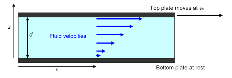
Just as for kinetic friction between solids, to keep the top plate moving requires a steady force. Obviously, the force is proportional to the total amount of fluid being kept in motion, that is, to the total area of the top plate in contact with the fluid. The significant parameter is the horizontal force per unit area of plate, say. This clearly has the same dimensions as pressure (and so can be measured in Pascals) although it is physically completely different, since in the present case the force is parallel to the area (or rather to a line within it), not perpendicular to it as pressure is.
(Note for experts only: Actually, viscous drag and pressure are not completely unrelatedas we shall discuss later, the viscous force may be interpreted as a rate of transfer of momentum into the fluid, momentum parallel to the surface that is, and pressure can also be interpreted as a rate of transfer of momentum, but now perpendicular to the surface, as the molecules bounce off. Physically, the big difference is of course that the pressure doesn’t have to do any work to keep transferring momentum, the viscous force does.)
defines the coefficient of viscosity The SI units of are Pascal.seconds, or Pa.s.
A convenient unit is the milliPascal.second, mPa.s. (It happens to be close to the viscosity of water at room temperature.) Confusingly, there is another set of units out there, the poise, named after Poiseuilleusually seen as the centipoise, which happens to equal the millipascal.second! And, there’s another viscosity coefficient in common use: the kinetic viscosity, where is the fluid density. This is the relevant parameter for fluids flowing downwards gravitationally. But we’ll almost always stick with .
Here are some values of for common liquids:
| Liquid | Viscosity in mPa.s |
|---|---|
| Water at 0℃ | 1.79 |
| Water at 20℃ | 1.002 |
| Water at 100℃ | 0.28 |
| Glycerin at 0℃ | 12070 |
| Glycerin at 20℃ | 1410 |
| Glycerin at 30℃ | 612 |
| Glycerin at 100℃ | 14.8 |
| Mercury at 20℃ | 1.55 |
| Mercury at 100℃ | 1.27 |
| Motor oil SAE 30 | 200 |
| Motor oil SAE 60 | 1000 |
| Ketchup | 50,000 |
Some of these are obviously ballpark the others probably shouldn’t be trusted to be better that 1% or so, glycerin maybe even 5-10% (see CRC Tables); these are quite difficult measurements, very sensitive to purity (glycerin is hygroscopic) and to small temperature variations.
To gain some insight into these very different viscosity coefficients, we’ll try to analyze what’s going on at the molecular level.
A Microscopic Picture of Viscosity in Laminar Flow
For Newton’s picture of a fluid sandwiched between two parallel plates, the bottom one at rest and the top one moving at steady speed, the fluid can be pictured as made up of many layers, like a pile of printer paper, each sheet moving a little faster than the sheet below it in the pile, the top sheet of fluid moving with the plate, the bottom sheet at rest. This is called laminar flow: laminar just means sheet (as in laminate, when a sheet of something is glued to a sheet of something else). If the top plate is gradually speeded up, at some point laminar flow becomes unstable and turbulence begins. We’ll assume here that we’re well below that speed.
So where’s the friction? It’s not between the fluid and the plates (or at least very little of it isthe molecules right next to the plates mostly stay in place) it’s between the individual sheetsthroughout the fluid. Think of two neighboring sheets, the molecules of one bumping against their neighbors as they pass. As they crowd past each other, on average the molecules in the faster stream are slowed down, and those in the slower stream speeded up. Of course, momentum is always conserved, but the macroscopic kinetic energy of the sheets of fluid is partially losttransformed into heat energy.
Exercise: Suppose a mass of fluid moving at in the -direction mixes with a mass moving at in the -direction. Momentum conservation tells us that the mixed mass moves at Prove that the total kinetic energy has decreased if are unequal.
This is the fraction of the kinetic energy that has disappeared into heat.
This molecular picture of sheets of fluids moving past each other gives some insight into why viscosity decreases with temperature, and at such different rates for different fluids. As the molecules of the faster sheet jostle past those in the slower sheet, remember they are all jiggling about with thermal energy. The jiggling helps break them loose if they get jammed temporarily against each other, so as the temperature increases, the molecules jiggle more furiously, unjam more quickly, and the fluid moves more easilythe viscosity goes down.
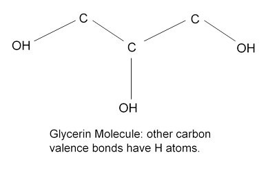
This drop in viscosity with temperature is dramatic for glycerin. A glance at the molecule suggests that the zigzaggy shape might cause jamming, but the main cause of the stickiness is that the outlying H’s in the OH groups readily form hydrogen bonds (see Atkins’ Molecules, Cambridge).
For mercury, a fluid of round atoms, the drop in viscosity with temperature is small. Mercury atoms don’t jam much, they mainly just bounce off each other (but even that bouncing randomizes their direction, converting macroscopic kinetic energy to heat). Note that mercury is a little more viscous than water: this can only be understood properly with some detailed chemical analysis, mercury is a metal so the bonds are metallic, meaning delocalized electron states. Water molecules attract with hydrogen bonds. Unfortunately, we can't investigate this further here.
Another mechanism generating viscosity is the diffusion of faster molecules into the slower stream and vice versa. As discussed below, this is far the dominant factor in viscosity of gases, but is much less important in liquids, where the molecules are crowded together and constantly bumping against each other.
This temperature dependence of viscosity is a real problem in lubricating engines that must run well over a wide temperature range. If the oil gets too runny (that is, low viscosity) it will not keep the metal surfaces from grinding against each other; if it gets too thick, more energy will be needed to turn the axle. “Viscostatic” oils have been developed: the natural decrease of viscosity with temperature (“thinning”) is counterbalanced by adding polymers, long chain molecules at high temperatures that curl up into balls at low temperatures.
Oiling a Wheel Axle
The simple linear velocity profile pictured above is actually a good model for ordinary lubrication. Imagine an axle of a few centimeters diameter, say about the size of a fist, rotating in a bearing, with a 1 mm gap filled with SAE 30 oil, having (Note: mPa, millipascals, not Pascals! 1Pa = 1000mPa.)
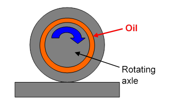
If the total cylindrical area is, say, 100 sq cm., and the speed is 1 m.s-1, the force per unit area (sq. m.)
So for our 100 sq.cm bearing the force needed to overcome the viscous “friction” is At the speed of 1 m sec-1, this means work is being done at a rate of 2 joules per sec., or 2 watts, which is heating up the oil. (This heat must be conducted away, or the oil continuously changed by pumping, otherwise it will get too hot.)
*Viscosity: Kinetic Energy Loss and Momentum Transfer
So far, we’ve viewed the viscosity coefficient as a measure of friction, of the dissipation into heat of the energy supplied to the fluid by the moving top plate. But is also the key to understanding what happens to the momentum the plate supplies to the fluid.
For the picture above of the steady fluid flow between two parallel plates, the bottom plate at rest and the top one moving, a steady force per unit area in the -direction applied to the top plate is needed to maintain the flow.
From Newton’s law is the rate at which momentum in the -direction is being supplied (per unit area) to the fluid. Microscopically, molecules in the immediate vicinity of the plate either adhere to it or keep bouncing against it, picking up momentum to keep moving with the plate (these molecules also constantly lose momentum by bouncing off other molecules a little further away from the plate).
Question: But doesn’t the total momentum of the fluid stay the same in steady flow? Where does the momentum fed in by the moving top plate go?
Answer: the -direction momentum supplied at the top passes downwards from one layer to the next, ending up at the bottom plate (and everything it’s attached to). Remember that, unlike kinetic energy, momentum is always conservedit can’t disappear.
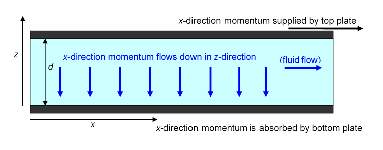
So, there is a steady flow in the -direction of -direction momentum. Furthermore, the left-hand side of the equation
is just this momentum flow rate. The right hand side is the coefficient of viscosity multiplied by the gradient in the -direction of the -direction velocity.
Viewed in this way, is a transport equation. It tells us that the rate of transport of -direction momentum downwards is proportional to the rate of change of -direction velocity in that direction, and the constant of proportionality is the coefficient of viscosity. And, we can express this slightly differently by noting that the rate of change of -direction velocity is proportional to the rate of change of -direction momentum density.
Recall that we mentioned earlier the so-called kinetic viscosity coefficient, Using that in the equation
replaces the velocity gradient with an -direction momentum gradient. To abbreviate a clumsy phrase, let’s call the -direction momentum density and the current of this in the -direction Then our equation becomes
The current of in the -direction is proportional to how fast is changing in that direction.
This closely resembles heat flowing from a hot spot to a cold spot: heat energy flows towards the place where there is less of it, “downhill” in temperature. The rate at which it flows is proportional to the temperature gradient, and the constant of proportionality is the thermal conductivity (see later). Here, the momentum flow is analogous: it too flows to where there is less of it, and the kinetic viscosity coefficient corresponds to the thermal conductivity.