 ----------------------------Eqn.(1)
POISEUILLE'S LAW AND THE VISCOSITY OF FLUIDS
INTRODUCTION
The simplest model for the flow of a fluid through a pipe is contained in Bernoulli's equation, which is simply an application of the law of conservation of mechanical energy to a moving fluid:
 ----------------------------Eqn.(1)
here P is the pressure of the fluid, r its density, h its height and v its velocity. This model assumes that the fluid is incompressible and that it suffers no friction as it moves through the pipe. The use of a single value for v in Bernoulli's law indicates that it is based on the assumption that every portion of the fluid moves with the same velocity. In reality that is clearly not the case: the part of the fluid that is in direct contact with the wall will move very slowly while elsewhere the velocity will be higher. The internal friction that causes this velocity gradient is called the viscosity of the fluid.
For sufficiently small velocities the flow will be laminar i.e. layered. One can show that laminar flow leads to a parabolic distribution of velocities across a pipe with a circular cylindrical cross section. As the velocity increases past a critical value, depending upon the viscosity and density of the fluid, eddies appear and the flow becomes turbulent.
The laminar flow through a pipe is described by the Hagen-Poiseuille law, stating that the flow rate (F = volume of fluid flowing per unit time) is proportional to the pressure difference Dp between the ends of the pipe and the fourth power of its radius r.
 ----------------------------------Eqn.(2)
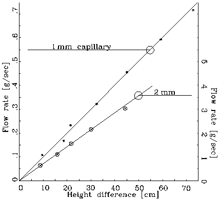
here l is the length of the pipe and m the coefficient of viscosity, a constant characteristic of the given fluid. It should be noted that, for liquids the coefficient of viscosity decreases, i.e., the liquid becomes less viscous, with increasing temperature. (We make here a distinction between a fluid, any medium that can flow, including gases, and liquids such as water. Experimentally, one can measure the coefficient of viscosity of a given liquid by observing its flow rate through a pipe of a given diameter under the effect of a known pressure. Obviously, the measurement should be performed while dealing with laminar, not turbulent flow: the presence of such a condition can be verified by observing the proportionality between flow rate and applied pressure. As shown in Fig.1, the onset of turbulent flow is indicated by a departure from the linear behavior.

Figure 1: Linear dependence of flow rate.
Note the strong (fourth power) dependence of the flow rate on
the pipe radius: even a small variation of the radius will cause
a large variation of the flow rate. Ergo, don't be too disturbed
by deviations from the r4 law that you
might observe: a 5% deviation from the given radius of the pipe
will lead to a 20% change in the flow rate.
Because the flowrate F and the pressure p are proportional to each other (Eq. 2) - as are current and voltage in Ohm's law - it is convenient to write Eq. 2 in a form analogous to Ohm's law by introducing the flow resistance R, defined as:
 . ----------------------------Eqn.(3)
APPARATUS
Water bottle; bottle stand; plastic tube; clamp; set of 3 capillary
tubes of different diameters; various adapters; stand and clamps
for capillaries; basin; beaker; funnel; meter stick; spirit level;
timer; scales; lab jack..
WHAT TO DO
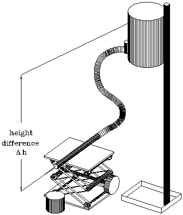
Figure 2 shows a schematic of the apparatus.
 Figure 2: Apparatus
1). Insert the 2 mm capillary into the end of the plastic tube and tape it to the lab jack with masking tape. Make sure the capillary is level, i.e. don't let the plastic tube rest on the jack. Fill the bottle with water and mount it so that the fluid level is 5 to 10 cm above the capillary. The height difference between the two determines the pressure difference
 ------------------------Eqn.(4)
which, in turn, determines the flow rate.
2). Dry the plastic beaker and the pans of the scale. Weigh
the empty beaker.
3). Start the water flow, making sure that the stopcock (the hose
clamp) is fully open and that there are no air bubbles moving
through the capillary. Holding the stop watch in one hand and
the dry beaker in the other, insert the latter into the water
stream while starting the former. Collect some 20 to 40 cm3
of water and withdraw the beaker while stopping the watch. Then,
immediately, stop the water flow by shutting the stopcock (the
hose clamp).
4). Measure the height difference, Dh,
between the water level in the bottle and the axis of the capillary.
5). Weigh the amount of water that you have collected and calculate
the flow rate F, taking the density of water to be 1 g/cm3.
6). Pour the collected amount of water back into the bottle and
measure the change in the water level. If necessary make a correction
by extrapolating to the level difference during the middle of
the flow rate measurement.
7). Plot the flow rate as a function of the height difference.
8). Dry the beaker and the scale.
9). Raise the bottle to a new level and go back to step 3.
10). Repeat steps 3) to 9) until you have reached the full height
of the stand or until the last point shows a clear deviation from
a linear depency on the pressure difference.
11). Repeat the entire procedure first for the 1.5 and then for
the 1 mm capillary. As the diameter decreases, it may be necessary
to start the measurements at a larger initial value of the height
difference and, for the smallest pipe, to collect the water for
up to two minutes.
In your lab report determine for each capillary the value
of m. Are the fluctuations of the individual
values consistent with the accuracy of the measurements? Calculate
for each capillary the flow resistance R = p/F, and plot it versus
r-4; according to Poiseuille's law you should get a
linear dependence, do you? In actuality you measure the flow resistance
of the capillary in series with the plastic tubing. Is this an
effect to be taken into account? How would this effect manifest
itself? How can you correct for it?