Classical Wave Equations
Michael Fowler
University of Virginia
Physics 252 Home Page
Link to Previous Lecture
Introduction
The aim of this section is to give a fairly brief review of waves in various shaped elastic media—beginning with a taut string, then going on to an elastic sheet, a drumhead, first of rectangular shape then circular, and finally considering elastic waves on a spherical surface, like a balloon.
The reason we look at this material here is that these are "real waves", hopefully not too difficult to think about, and yet mathematically they are the solutions of the same wave equation the Schrödinger wave function obeys in various contexts, so should be helpful in visualizing solutions to that equation, in particular for the hydrogen atom.
We begin with the stretched string, then go on to the rectangular and circular drumheads. We derive the wave equation from F = ma for a little bit of string or sheet. The equation corresponds exactly to the Schrödinger equation for a free particle with the given boundary conditions.
The most important section here is the one on waves on a sphere. We find the first few standing wave solutions. These waves correspond to Schrödinger’s wave function for a free particle on the surface of a sphere. This is what we need to analyze to understand the hydrogen atom, because using separation of variables we split the electron’s motion into radial motion and motion on the surface of a sphere. The potential only affects the radial motion, so the motion on the sphere is free particle motion, described by the same waves we find for vibrations of a balloon.
Waves on a String
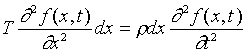
Let’s begin by reminding ourselves of the wave equation for waves on a taut string, stretched between x = 0 and x = L, tension T newtons, density
r kg/meter. Assuming the string’s equilibrium position is a straight horizontal line (and, therefore, ignoring gravity), and assuming it oscillates in a vertical plane, we use f(x,t) to denote its shape at instant t, so f(x,t) is the instantaneous upward displacement of the string at position x. We assume the amplitude of oscillation remains small enough that the string tension can be taken constant throughout.The wave equation is derived by applying F = ma to an infinitesimal length dx of string. We picture our little length of string as bobbing up and down in simple harmonic motion, which we can verify by finding the net force on it as follows. At the left hand end of the string, point x, say, the tension T is at a small angle df(x)/dx to the horizontal, since the tension acts necessarily along the line of the string. Since it is pulling to the left, there is a downward force component Tdf(x)/dx. At the right hand end of the string fragment there is an upward force Tdf(x + dx)/dx. Putting f(x + dx) = f(x) + (df/dx)dx, and adding the almost canceling upwards and downwards forces together, we find a net force T(d2f/dx2)dx on the bit of string. The string mass is
r dx, so F = ma becomes
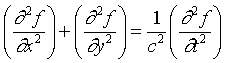
giving the standard wave equation
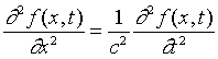
with wave velocity given by c2 = T/r .
This equation can of course be solved by separation of variables, f(x,t) = f(x)g(t), and the equation for f(x) is identical to the time independent Schrödinger equation for a particle confined to (0,L) by infinitely high walls at the two ends. This is why the eigenfunctions (states of definite energy) for a Schrödinger particle confined to (0,L) are identical to the modes of vibration of a string held between those points. (However, it should be realized that the time dependence of the string wave equation and the Schrödinger time-dependent equation are quite different, so a nonstationary state, one corresponding to a sum of waves of different energies, will develop differently in the two systems.)
Waves on a Rectangular Drumhead
Let us now move up to two dimensions, and consider the analogue to the taut string problem, which is waves in a taut horizontal elastic sheet, like, say, a drumhead. Let us assume a rectangular drumhead to begin with. Then, parallel to the argument above, we would apply F = ma to a small square of elastic with sides parallel to the x and y axes. The tension from the rest of the sheet tugs along all four sides of the little square, and we realize that tension in a sheet of this kind must be defined in newtons per meter, so the force on one side of the little square is given by multiplying this "tension per unit length" by the length of the side.
Following the string analysis, we take the vertical displacement of the sheet at instant t to be given by f(x,y,t). We assume this displacement is quite small, so the tension itself doesn’t vary, and that each bit of the sheet oscillates up and down (the sheet is not tugged to one side). Suppose the bottom left-hand corner (so to speak) of the square is (x,y), the top right-hand corner (x + dx, y + dy). Then the left and right edges of the square have lengths dy. Now, what is the total force on the left edge? The force is Tdy, in the local plane of the sheet, perpendicular to the edge dy. Factoring in the slope of the sheet in the direction of the force, the vertically downward component of the force must be Tdy
¶ f(x,y,t)/¶ x. By the same argument, the force on the right hand edge has to have an upward component Tdy ¶ f(x+dx,y,t)/¶ x.Thus the net upward force on the little square from the sheet tension tugging on its left and right sides is
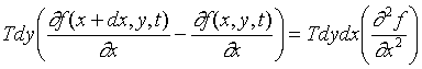
The net vertical force from the sheet tension on the other two sides is the same with x and y interchanged.
The mass of the little square of elastic sheet is
r dxdy, and its upward acceleration is ¶ 2f/¶ t2. Thus F = ma becomes:![]()
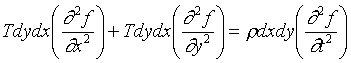
giving
with c2 = T/r .
This equation can be solved by separation of variables, and the time independent part is identical to the Schrödinger time independent equation for a free particle confined to a rectangular box.
Waves on a Circular Drumhead
A similar argument gives the wave equation for a circular drumhead, this time in (r,
j ) coordinates (we use j rather than q here because of its parallel role in the spherical case, to be discussed shortly).This time, instead of a tiny square of elastic, we take the small area rdrd
j bounded by the circles of radius r and r + dr and lines through the origin at angles j and j + dj . Now, the downward force from the tension T in the sheet on the inward curved edge, which has length rdj , is Trdj .¶ f(r, j , t)/¶ r. On putting this together with the upward force from the other curved edge, it is important to realize that the r in Trdj varies as well as ¶ f/¶ r on going from r to r + dr, so the sum of the two terms is Tdj ¶ /¶ r(r¶ f/¶ r)dr. To find the vertical elastic forces from the straight sides, we need to find how the sheet slopes in the direction perpendicular to those sides. The measure of length in that direction is not j , but rj , so the slope is 1/r.¶ f/¶ j , and the net upward elastic force contribution from those sides (which have length dr) is Tdrdj ¶ /¶ j (1/r.¶ f/¶ j ).Writing F = ma for this small area of elastic sheet, of mass
r rdrdj , gives then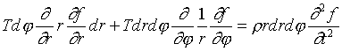
which can be written
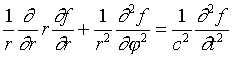
This is the wave equation in polar coordinates. Separation of variables gives a radial equation called Bessel’s equation, the solutions are called Bessel functions. These are what we encountered in describing an electron captured in a circular corral on a surface.
Waves on a Spherical Balloon
Finally, let us consider elastic waves on the surface of a sphere, such as an inflated spherical balloon. The natural coordinate system here is spherical polar coordinates, with
q measuring latitude, but counting the north pole as zero, the south pole as p . The angle j measures longitude from some agreed origin.We take a small elastic element bounded by longitude lines
j and j + dj and latitude q and q + dq . For a sphere of radius r, the sides of the element have lengths rsinq dj , rdq , etc. Beginning with one of the longitude sides, length rdq , tension T, the only slightly tricky point is figuring its deviation from the local horizontal, which is 1/rsinq .(¶ f/¶ j ), since increasing j by dj means moving an actual distance rsinq dj on the surface, just analogous with the circular case above. Hence, by the usual method, the actual vertical force from tension on the two longitude sides is Trdq dj . (¶ /¶ j )1/rsinq .(¶ f/¶ j ).To find the force on the latitude sides, taking the top one first, the slope is given by 1/r.
¶ f/¶ q , so the force is just Trsinq dj .1/r.¶ f/¶ q . On putting this together with the opposite side, it is necessary to recall that sinq as well as f varies with q , so the sum is given by: Trdj dq ¶ /¶ q sinq .1/r.¶ f/¶ q . We are now ready to write down F = ma once more, the mass of the element is r r2sinq dq dj . Canceling out elements common to both sides of the equation, we find: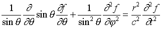 .
.
Again, this wave equation is solved by separation of variables. The time independent solutions are called the Legendre functions. They are the basis for analyzing the vibrations of any object with spherical symmetry, for example a planet struck by an asteroid, or vibrations in the sun generated by large solar flares.
Simple Solutions to the Spherical Wave Equation
Recall that for the two dimensional circular case, after separation of variables the angular dependence was all in the solution to
¶ 2f/¶ j 2 = -l f, and the physical solutions must fit smoothly around the circle (no kinks, or it would not satisfy the wave equation at the kink), leading to solutions sinmj and cosmj (or eimj ) with m an integer, and l = m2 (this is why we took l with a minus sign in the first equation).For the spherical case, the equation containing all the angular dependence is
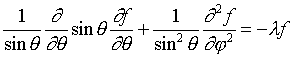
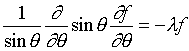
The standard approach here is, again, separation of variables. Taking the first term on the left hand side over to the right, and multiplying throughout by sin2q isolates the j term:
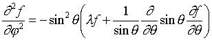
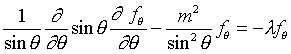
Writing now f(q ,j ) = fq (q )fj (j ) in the above equation, and dividing throughout by f, we find as usual that the left hand side depends only on j , the right hand side only on q , so both sides must be constants. Taking the constant as -m2, the j solution is e± imj , and one can insert that in the q equation to give
Obviously, f = constant is a solution with eigenvalue l = 0.
What about possible solutions that don’t depend on j ? The equation would be the simpler
Try f = cosq . It is easy to check that this is a solution, with l = 2.
Try f = sinq . This is not a solution. In fact, we should have realized it cannot be a solution to the wave equation by visualizing the shape of the elastic sheet near the north pole. If f = sinq , f = 0 at the pole, but rises linearly (for small q ) going away from the pole. Thus the pole is at the bottom of a conical valley. But this conical valley amounts to a kink in the elastic sheet—the slope of the sheet has a discontinuity if one moves along a line passing through the pole, so the shape of the sheet cannot satisfy the wave equation at that point. This is somewhat obscured by working in spherical coordinated centered there, but locally the north pole is no different from any other point on the sphere, we could just switch to local (x,y) coordinates, and the cone configuration would clearly not satisfy the wave equation.
However, f = sinq sinj is a solution to the equation. It is a worthwhile exercise to see how the j term gets rid of the conical point at the north pole by considering the value of f as the north pole is approached for various values of j : j = 0, p /2, p , 3p /2 say. The sheet is now smooth at the pole!
We find f = sinq cosj , sinq sinj (and so sinq eij ) are solutions with l = 2.
It is straightforward to verify that f = cos2q - 1/3 is a solution with l = 6.
Finally, we mention that other l = 6 solutions are sinq cosq sinj and sin2q sin2j .
We do not attempt to find the general case here, but we have done enough to see the beginnings of the pattern. We have found the series of eigenvalues 0, 2, 6, … . It turns out that the complete series is given by l = l(l + 1), with l = 0, 1, 2, … . This integer l is the analogue of the integer m in the wave on a circle case. Recall that for the wave on the circle, if we chose real wave functions (cosmj , sinmj not eimj ) then 2m gave the number of nodes the wave had (that is, m complete wavelengths fitted around the circle). It turns out that on the sphere l gives the number of nodal lines (or circles) on the surface. This assumes that we again choose the j component of the wave function to be real, so that there will be m nodal circles passing through the two poles corresponding to the zeros of the cosmj term. We find that there are l - m nodal latitude circles corresponding to zeros of the function of q .
Summary: First Few Standing Waves on the Balloon
l l m form of solution (unnormalized)
0 0 0 constant
2 1 0 cos
q2 1 1 sin
q eij2 1 -1 sin
q e-ij6 2 0 cos2
q - 1/36 2
± 1 cosq sinq e± ij6 2 ± 2 sin2qe± 2ij
The Schrödinger Equation for the Hydrogen Atom
How Do We Separate the Variables?
In three dimensions, the Schrödinger equation for an electron in a potential can be written:
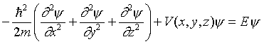
This is the obvious generalization of our previous two-dimensional discussion, and we will later be using the equation in the above form to discuss electron wave functions in metals, where the standard approach is to work with standing waves in a rectangular box.
Recall that in our original "derivation" of the Schrödinger equation, by analogy with the Maxwell wave equation for light waves, we argued that the differential wave operators arose from the energy-momentum relationship for the particle, that is
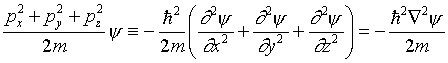
so that the time-independent Schrödinger wave equation is nothing but the statement that E = K.E. + P.E. with the kinetic energy expressed as the equivalent operator.
To make further progress in solving the equation, the only trick we know is separation of variables. Unfortunately, this won’t work with the equation as given above in (x, y, z) coordinates, because the potential energy term is a function of x, y and z in a nonseparable form. The solution is, however, fairly obvious: the potential is a function of radial distance from the origin, independent of direction. Therefore, we need to take as our coordinates the radial distance r and two parameters fixing direction, q and j . We should then be able to separate the variables, because the potential only affects radial motion. No potential term will appear in the equations for q , j motion, that will be free particle motion on the surface of a sphere.
Momentum and Angular Momentum with Spherical Coordinates
It is worth thinking about what are the natural momentum components for describing motion in spherical polar coordinates (r,
q , j ). The radial component of momentum, pr, points along the radius, of course. The q component pq points along a line of longitude, away from the north pole if positive (remember q itself measures latitude, counting the north pole as zero). The j momentum component, pj , points along a line of latitude.It will be important in understanding the hydrogen atom to connect these momentum components (pr, p
q , pj ) with the angular momentum components of the atom. Evidently, momentum in the r-direction, which passes directly through the center of the atom, contributes nothing to the angular momentum. Consider now a particle for which pr = pq = 0, only pj being nonzero. Classically, such a particle is circling the north pole at constant latitude q , say, so it is moving in space in a circle or radius rsinq in a plane perpendicular to the north-south axis of the sphere. Therefore, it has an angular momentum about that axis![]() , say.
, say.
(The standard transformation from (x, y, z) coordinates to (r, q , j ) coordinates is to take the north pole of the q , j sphere to be on the z-axis.)
As we shall see in detail below, the wave equation describing the j motion is a simple one, with solutions of the form eimj with integer m, just as in the two-dimensional circular well. This just means that the component of angular momentum along the z-axis is quantized, ![]() , with m an integer.
, with m an integer.
Total Angular Momentum and Waves on a Balloon
The total angular momentum is L = rp
^ , where p^ is the component of the particle’s momentum perpendicular to the radius, so p^ 2 = pj 2 + pq 2. Thus the square of the total angular momentum is (apart from a constant factor) the kinetic energy of a particle moving freely on the surface of a sphere. The equivalent Schrödinger equation for such a particle is the wave equation given in the last section for waves on a balloon. (This can be established by the standard change of variables routine on the differential operators). Therefore, the solutions we found for elastic waves on a sphere actually describe the angular momentum wave function of the hydrogen atom. We conclude that the total angular momentum is quantized,Angular Momentum and the Uncertainly Principle
The conclusions of our above waves on a sphere analysis of the angular momentum of a quantum mechanical particle are a little strange. We found that the component of angular momentum in the z-direction must be a whole number of ![]() units, yet the square of the total angular momentum
units, yet the square of the total angular momentum ![]() is not a perfect square! One might wonder if the component of angular momentum in the x-direction isn’t also a whole number of
is not a perfect square! One might wonder if the component of angular momentum in the x-direction isn’t also a whole number of ![]() units as well, and if not, why not? The key is that in questions of this type we are forgetting the essentially wavelike nature of the particle’s motion, or, equivalently, the uncertainty principle. Recall first that the z-component of angular momentum, that is, the angular momentum about the z-axis, is the product of the particle’s momentum in the xy-plane and the distance of the line of that motion from the origin. There is no contradiction in specifying that momentum and that position simultaneously, because they are in perpendicular directions. However, we cannot at the same time specify either of the other components of the angular momentum, because that would involve measuring some component of momentum in a direction in which we have just specified a position measurement. We can measure the total angular momentum, that involves additionally only the component p
units as well, and if not, why not? The key is that in questions of this type we are forgetting the essentially wavelike nature of the particle’s motion, or, equivalently, the uncertainty principle. Recall first that the z-component of angular momentum, that is, the angular momentum about the z-axis, is the product of the particle’s momentum in the xy-plane and the distance of the line of that motion from the origin. There is no contradiction in specifying that momentum and that position simultaneously, because they are in perpendicular directions. However, we cannot at the same time specify either of the other components of the angular momentum, because that would involve measuring some component of momentum in a direction in which we have just specified a position measurement. We can measure the total angular momentum, that involves additionally only the component p
Thus the uncertainty principle limits us to measuring at the same time only the total angular momentum and the component in one direction. Note also that if we knew the z-component of angular momentum to be m![]() , and the total angular momentum were
, and the total angular momentum were ![]() with l = m, then we would also know that the x and y components of the angular momentum were exactly zero. Thus we would know all three components, in contradiction to our uncertainly principle arguments. This is the essential reason why the square of the total angular momentum is greater than the maximum square of any one component. It is as if there were a "zero point motion" fuzzing out of the direction.
with l = m, then we would also know that the x and y components of the angular momentum were exactly zero. Thus we would know all three components, in contradiction to our uncertainly principle arguments. This is the essential reason why the square of the total angular momentum is greater than the maximum square of any one component. It is as if there were a "zero point motion" fuzzing out of the direction.
Another point related to the uncertainty principle concerns measuring just where in its circular (say) orbit the electron is at any given moment. How well can that be pinned down? There is an obvious resemblance here to measuring the position and momentum of a particle at the same time, where we know the fuzziness of the two measurements is related by
D p.D x ~ h. Naïvely, for a circular orbit of radius r in the xy-plane, pr = Lz and distance measured around the circle is rq , so D p.D x ~ h suggests D Lz.D q ~ h. That is to say, precise knowledge of Lz implies no knowledge of where on the circle the particle is. This is nor surprising, because we have found that for Lz = mThe Schrödinger Equation in (r,
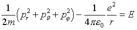
q , j ) CoordinatesIt is worth writing first the energy equation for a classical particle in the Coulomb potential:
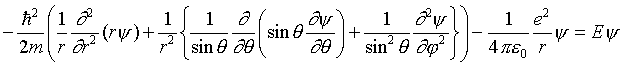
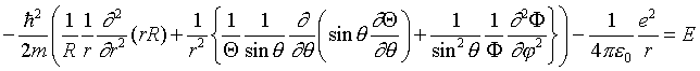
This makes it possible to see, term by term, what the various parts of the Schrödinger equation signify. In spherical polar coordinates, Schrödinger’s equation is:
Separating the Variables: the Messy Details
We look for separable solutions of the form
![]()
We now follow the standard technique. That is to say, we substitute RQ F for y in each term in the above equation. We then observe that the differential operators only actually operate on one of the factors in any given part of the expression, so we put the other two factors to the left of these operators. We then divide the entire equation by RQ F , to get
Separating Out and Solving the
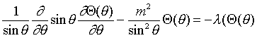
F (j ) EquationThe above equation can be rearranged to give:
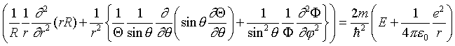
Further rearrangement leads to:
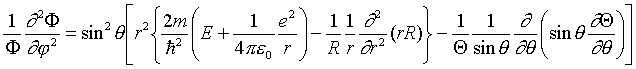
At this point, we have achieved the separation of variables! The left hand side of this equation is a function only of
j , the right hand side is a function only of r and q . The only way this can make sense is if both sides of the equation are in fact constant (and of course equal to each other).Taking the left hand side to be equal to a constant we denote for later convenience by -m2,
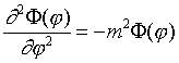
We write the constant -m2 because we know that as a factor in a wave function
F (j ) must be single valued as j increases through 2p , so an integer number of oscillations must fit around the circle, meaning F is sinmj , cosmj or eimj with m an integer. These are the solutions of the above equation. Of course, this is very similar to the particle in the circle in two dimensions, m signifies units of angular momentum about the z-axis.Separating Out the
Q (q ) EquationBacking up now to the equation in the form
we can replace the  term by -m2, and move the r term over to the right, to give
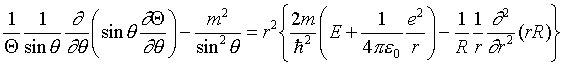
We have again managed to separate the variables—the left hand side is a function only of q , the right hand side a function of r. Therefore both must be equal to the same constant, which we set equal to -l .
This gives the Q (q ) equation:
![]()
This is exactly the wave equation we discussed above for the elastic sphere, and the allowed eigenvalues l are l(l+1), where l = 0, 1, 2, .. with l ³ m.
The R(r) Equation
Replacing the
q ,j operator with the value found just above in the original Schrödinger equation gives the equation for the radial wave function: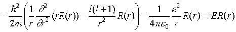
The first term in this radial equation is the usual radial kinetic energy term, equivalent to pr2/2m in the classical picture. The third term is the Coulomb potential energy. The second term is an effective potential representing the centrifugal force. This is clarified by reconsidering the energy equation for the classical case,
The angular momentum is ![]() . Thus for fixed angular momentum, we can write the above "classical" equation as
. Thus for fixed angular momentum, we can write the above "classical" equation as
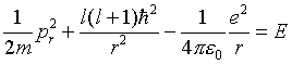
The parallel to the radial Schrödinger equation is then clear.
We must find the solutions of the radial Schrödinger equation that decay for large r. These will be the bound states of the hydrogen atom. Following French (p 521 of Quantum Mechanics) we go to natural units, measuring lengths in units of the first Bohr radius, and energies in Rydberg units
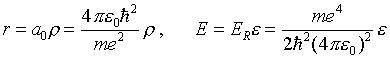 .
.
Finally taking u(r) = rR(r)
the radial equation becomes
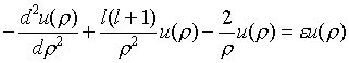 .
.
Physics 252 Home Page Copyright
Link to Next Lecture