581 home 152 home Lecture on Simple Pendulum PDF

Spreadsheet Treatment of the Simple Pendulum

Michael Fowler, University of Virginia

Equation of Motion

Let’s consider a simple pendulum but with the string replaced by a light rod, so that it can swing through really large angles, even up to the top. Let us further assume that the end of the rod away from the bob is attached to a collar free to rotate about a frictionless horizontal rod, so that the pendulum is constrained to move along a fixed vertical circle (it can’t swing "sideways").

We take the length of the pendulum to be L, the mass of the bob m and the masses of the rod (and collar) negligible. The position of the pendulum on the circle is labeled by θ , with vertically downward being θ = 0. We will measure θ in radians. The angular velocity we call ω (omega), so w is the rate of change of θ with time, measured in radians per second. Thus the actual velocity of the pendulum bob is Lw meters per second along the circle.

The component of the gravitational force moving the pendulum along the circle is mgsinθ . We are not going to replace this by mgθ this time, because we want to be able to analyze the case where the pendulum swings through large angles.

The equation of motion is:

Note that m cancels on the two sides, as we expect.

First Attempt at Solving the Equation of Motion

As usual, we begin at time t = 0, and track how the system changes in time steps Δt. We approximate the position at time by:

This is clearly an approximation: we would be better off taking w(t) somewhere inside the interval rather than right at the beginning, since it will be varying. The hope is that if we take the interval sufficiently small, this will not lead to much error.

We approximate the change in angular speed over the interval by

where we denote the angular acceleration by α(t). This angular acceleration is of course given by the equation of motion.

The above equations contain enough information to construct a spreadsheet to track the movements of the pendulum.

As usual, we name a series of squares (say, B15 through B19) for the variables we need, L, g, theta_init, omega_init and delta_t. We first write L= in A15, g= in A16, and so on down to A19, then in B15 click Insert Name Define. Excel will suggest L, click OK.

Put the following set of values in B15 through B19: L = 1, g = 10, theta_init = 0, omega_init = 1, delta_t = 0.01.

Now, in A22, B22, C22 and D22 write time, theta, omega, accn respectively.

In A23 write 0, and in A24 write =A23 + delta_t.

In B23 write =theta_init, in C23 write =omega_init, and in D23 write =-(g/L)*sin(B23).

In B24 write =B23 + C23*delta_t, in C24 write =C23 + D23*delta_t, and D24 =-(g/L)*sin(B24).

Pause at this point to be sure you understand why these entries are equivalent to the formulas for θ(t + Δ t) and w (t + Δ t) given above.

Now, select the four squares A24 through D24, and copy them down 200 rows by dragging with the cursor on the bottom right hand corner of the selected squares, so that the white cross or arrow changes into a small black cross.

Next, select the relevant data in the first two columns (200 rows of time and theta), click Chart Wizard, and choose xy scatter graph. With the parameter values suggested above, you should see about one period of a sine wave, which looks fairly satisfactory.

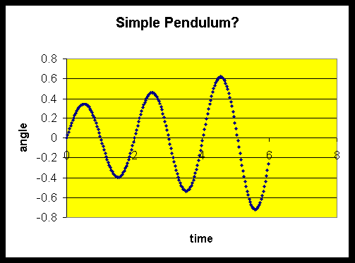
Now change delta_t to 0.03. This should give:

This is definitely not good news! Our equations are supposed to describe a very ordinary pendulum, but this one seems to have a hidden source of energy!

A Better Approximation: the Leapfrog

The problem is that our approximations were just not good enough, and the errors evidently build up as time goes along. We must improve on the equations:

and

The best way to improve them would be to have values of w (t) and a (t) more representative of the whole interval, not just the first point in the interval.

A much more accurate set of equations would be:

and

The "leapfrog" method is a way of making a small change in the spreadsheet you’ve already constructed so that it calculates using this new improved set of equations.

The basic trick is to continue as before finding θ and α at times θ, Δ t, 2Δ t, 3Δ t and so on, BUT to find the velocity w at times ½Δ t, 1½Δ t, 2½Δ t, etc.

(This is slightly awkward for the very first step, but then it’s OK.)

So in the first row after the initial one, we put in values t + Δ t, θ (t + Δ t), w(t + ½Δ t), α(t + Δ t). The important difference, of course, is that we have only advanced w by half the time interval, so we write in C24: =C23+0.5*D23*delta_t.

Perhaps it’s worth putting in a “timetable” showing explicitly the times corresponding to the values in each of the spreadsheet cells:

time	theta	omega	alpha
(A23) 0	B23: theta_init	C23: omega_init	D23
0.5*delta_t		C24
(A24) 1*delta_t	B24		D24
1.5*delta_t		C25
(A25) 2*delta_t	B25		D25

Now in B24 write: =B23+C24*delta_t. This means we are calculating the change in angle by using the angular velocity in the middle of the interval. Copy this formula down to B25 by dragging, and also drag down to row 25 the formula for time steps in column A and the formula for angular acceleration in column D.

The remaining important step is to write in C25: =C24+D24*delta_t. This means we are calculating the change in angular velocity by using the angular acceleration in the middle of the interval.

Now select the four cells A25 through D25 and copy down 200 rows by dragging the bottom right-hand corner in the usual fashion.

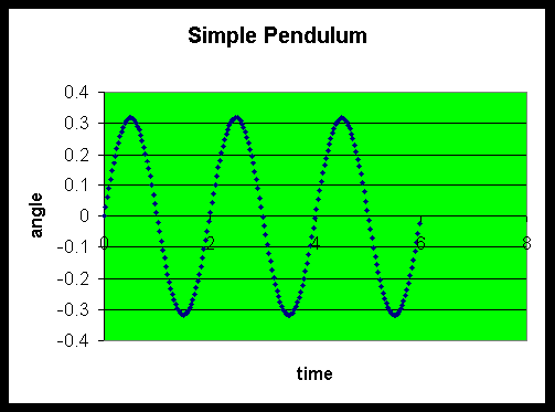
Taking the same values we used above, L = 1, g = 10, theta_init = 0, omega_init = 1, delta_t = 0.03 we find:

The improvement in accuracy is dramatic! This spreadsheet is now reliable enough to explore some interesting properties of the pendulum.

The presentation above parallels that for Lotus 1-2-3 in Spreadsheet Physics, by Misner and Cooney (1991).

Exercises

1. Plot angle and angular velocity on the same graph. Describe in words how the two curves relate to each other. (Is one the slope of the other?

The area under the other? Or what?)

2. Add another column to the spreadsheet in which you enter the total energy, potential + kinetic, at that time. This is a check on the accuracy of

the computation.

3. Keeping everything else constant, with L = 1 and g = 10, vary omega_init between 6 and 7, and interpret the graphs you get for θ as a function of t.

4. In exercise 3, you should have seen a big change in the shape of the curve at a particular value of omega_init. Can you work out that value by thinking about potential and kinetic energies? Use your result to check on the accuracy of the spreadsheet.