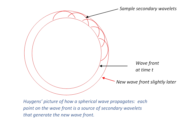
If a point source of light is switched on, the wavefront is an expanding sphere centered at the source. Huygens suggested that this could be understood if at any instant in time each point on the wavefront was regarded as a source of secondary wavelets, and the new wavefront a moment later was to be regarded as built up from the sum of these wavelets. For a light shining continuously, this process just keeps repeating.

What use is this idea? For one thing, it explains refraction—the change in direction of a wavefront on entering a different medium, such as a ray of light going from air into glass.
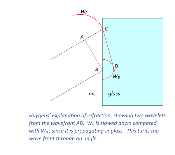
If the light moves more slowly in the glass, velocity v instead of c, with v < c, then Huygen’s picture explains Snell’s Law, that the ratio of the sines of the angles to the normal of incident and transmitted beams is constant, and in fact is the ratio c/v. This is evident from the diagram below: in the time the wavelet centered at A has propagated to C, that from B has reached D, the ratio of lengths AC/BD being c/v. But the angles in Snell’s Law are in fact the angles ABC, BCD, and those right-angled triangles have a common hypotenuse BC, from which the Law follows.

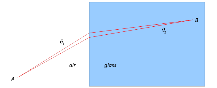
We will now temporarily forget about the wave nature of light, and consider a narrow ray or beam of light shining from point A to point B, where we suppose A to be in air, B in glass. Fermat showed that the path of such a beam is given by the Principle of Least Time: a ray of light going from A to B by any other path would take longer. How can we see that? It’s obvious that any deviation from a straight line path in air or in the glass is going to add to the time taken, but what about moving slightly the point at which the beam enters the glass?

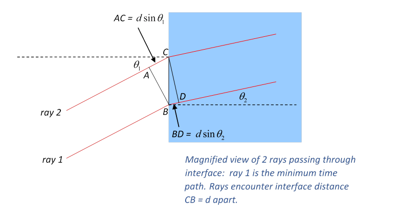
Where the air meets the glass, the two rays, separated by a small distance CD = d along that interface, will look parallel:

(Feynman gives a nice illustration: a lifeguard on a beach spots a swimmer in trouble some distance away, in a diagonal direction. He can run three times faster than he can swim. What is the quickest path to the swimmer?)
Moving the point of entry up a small distance d, the
light has to travel an extra
in air, but a distance
less by
in the glass, giving
an extra travel time
. For the classical
path, Snell’s Law gives
, so
to first order. But if we look at a series of possible paths,
each a small distance d away from the next at the point of crossing from
air into glass,
becomes of order d/c
away from the classical path.
Suppose now we imagine that the light actually travels along all these paths with about equal amplitude. What will be the total contribution of all the paths at B? Since the times along the paths are different, the signals along the different paths will arrive at B with different phases, and to get the total wave amplitude we must add a series of unit 2D vectors, one from each path. (Representing the amplitude and phase of the wave by a complex number for convenience—for a real wave, we can take the real part at the end.)
When we map out these unit 2D vectors, we find that in the neighborhood of the classical path,
the phase varies little, but as we go away from it the phase spirals more and
more rapidly, so those paths interfere amongst themselves destructively. To formulate this a little more precisely,
let us assume that some close by path has a phase difference φ from the least time path, and
goes from air to glass a distance x
away from the least time path: then for these close by paths,
, where a depends
on the geometric arrangement and the wavelength. From this, the sum over the close by paths is
an integral of the form
. (We are assuming the
wavelength of light is far less than the size of the equipment.) This is a standard integral, its value is
, all its weight is concentrated in a central area of width
, exactly as for the real function
.
This is the explanation of Fermat’s Principle—only near the path of least time do paths stay approximately in phase with each other and add constructively. So this classical path rule has an underlying wave-phase explanation. In fact, the central role of phase in this analysis is sometimes emphasized by saying the light beam follows the path of stationary phase.
Of course, we’re not summing over all paths here—we assume that the path in air from the source to the point of entry into the glass is a straight line, clearly the subpath of stationary phase.
Confining our attention for the moment to the mechanics of a single nonrelativistic particle in a potential, with Lagrangian L = T - V, the action S is defined by

With the advent of quantum mechanics, and the realization that any particle, including a thrown ball, has wave like properties, the rather mysterious Principle of Least Action looks a lot like Fermat’s Principle of Least Time. Recall that Fermat’s Principle works because the total phase along a path is the integrated time elapsed along the path, and for a path where that integral is stationary for small path variations, neighboring paths add constructively, and no other sets of paths do. If the Principle of Least Action has a similar explanation, then the wave amplitude for a particle going along a path from A to B must have a phase equal to some constant times the action along that path. If this is the case, then the observed path followed will be just that of least action, or, more generally, of stationary action, for only near that path will the amplitudes add constructively, just as in Fermat’s analysis of light rays.
Of course, if we write a phase factor for a path eicS where S is the action for the path and
c is some constant, c must necessarily have the dimensions of
inverse action. Fortunately, there is a natural candidate for the constant c. The wave nature of matter arises from quantum
mechanics, and the fundamental constant of quantum mechanics, Planck’s
constant, is in fact a unit of action.
(Recall action has the same dimensions as Et, and therefore the same as px,
manifestly the same as angular momentum.)
It turns out that the appropriate path phase factor is
.
That the phase factor is
, rather than
, say, can be established by considering the double slit
experiment for electrons (Peskin page 277).

This is analogous to the light waves going from a source in air to a point in glass, except now we have vacuum throughout (electrons don’t get far in glass), and we close down all but two of the paths.
Suppose electrons from the top slit, Path I, go a distance D
to the detector, those from the bottom slit, Path II, go D + d,
with d << D. Then if the electrons have wavelength
we know the phase
difference at the detector is
. To see this from our
formula for summing over paths, on Path I the action S = Et = ½mv12t,
and v1 = D/t, so
S1 = ½mD2/t.
For Path II, we must take v2 = (D + d)/t. Keeping only terms of leading order in d/D, the action difference between the two paths
S2 - S1 = mDd/t
So the phase difference
![]()
This is the known correct result, and this fixes the constant multiplying the action/h in the expression for the path phase.
In quantum mechanics, such as the motion of an electron in
an atom, we know that the particle does not follow a well-defined path, in
contrast to classical mechanics. Where
does the crossover to a well-defined path take place? Taking the simplest possible case of a free
particle (no potential) of mass m moving at speed v, the action
along a straight line path taking time t from A to B is ½mv2t.
If this action is of order Planck’s constant h, then the phase factor
will not oscillate violently on moving to different paths, and a range of paths
will contribute. In other words, quantum
rather than classical behavior dominates when ½mv2t is
of order h. But vt is the
path length L, and mv/h is the wavelength
, so we conclude that we must use quantum mechanics when the
wavelength h/p is significant compared with the path length. Interference sets in when the difference
in path actions is of order h, so in the atomic regime many paths must
be included.
Feynman (in Feynman and Hibbs) gives a nice picture to help think about summing over paths. He begins with the double slit experiment for an electron. We suppose the electron is emitted from some source A on the left, and we look for it at a point B on a screen to the right. In the middle is a thin opaque barrier with the familiar two slits. Evidently, to find the amplitude for the electron to reach B we sum over two paths. Now suppose we add another two-slit barrier. We have to sum over four paths. Now add another. Next, replace the two slits in each barrier by several slits. We must sum over a multitude of paths! Finally, increase the number of barriers to some large number N, and at the same time increase the number of slits to the point that there are no barriers left. We are left with a sum over all possible paths through space from A to B, multiplying each path by the appropriate action phase factor. This is reminiscent of the original wave propagation picture of Huygens: if one pictures it at successive time intervals of picoseconds, say, from each point on the wavefront waves go out 3 mm in all directions, then in the next time interval each of those sprouts more waves in all directions. One could write this as a sum over all zigzag paths with random 3 mm steps.
In fact, the sum over paths is even more daunting than Feynman’s picture suggests. All the paths going through these many slitted barriers are progressing in a forward direction, from A towards B. Actually, if we’re summing over all paths, we should be including the possibility of paths zigzagging backwards and forwards as well, eventually arriving at B. We shall soon see how to deal systematically with all possible paths.
As a warm up exercise, consider an electron confined
to one dimension, with no potential present, moving from
at time 0 to x
at time T. We’ll follow Feynman
in using T for the final time, so we
can keep t for the continuous (albeit
sometimes discretized) time variable over the interval 0 to T.
(As explained previously, when we write that the
electron is initially at
, we mean its wave function is a normalizable state, such as
a Gaussian, concentrated closely at
. The propagator then represents the probability amplitude,
that is, the wave function, at point x
after the given time T.) The propagator is given by
![]()
or, in Schrödinger wave function notation,
![]()
It is clear that for this to make sense, as ![]()
In the lecture on propagators, we found

Let us formulate the sum over paths for this simplest
one-dimensional case, the free electron, more precisely. Each path is a continuous function of time
in the time interval
, with boundary conditions
Each path contributes
a term
, where
![]()
(for the free electron case) evaluated along that path.
The integral over all paths is written:
![]()
This rather formal statement begs the question of how, exactly, we perform the sum over paths: what is the appropriate measure in the space of paths?
A natural approach is to measure the paths in terms of their
deviation form the classical path, since we know that dominates in the
classical limit. The classical path for
the free electron is just the straight line from
to x, traversed at constant velocity, since
there are no forces acting on the electron.
We write
![]()
where
![]()
and therefore
![]()
Then

The middle term on the bottom line is zero, as it has to be since it is a linear term in the deviation from the minimum path. To see this explicitly, one can integrate by parts: the end terms are zero, from the boundary condition on y, and the other term is the acceleration of the particle along the classical path, which is zero.
Therefore
![]()
The y-paths, being
the deviation from the classical path from
to x, necessarily
begin and end at the y-origin, since all paths summed over go from
to x.
The classical path, motion from
to x at a
constant speed
, has action Et,
with E the classical energy ½ mv2 , so
![]()
This gives the correct exponential term. The prefactor A, representing the sum
over the deviation paths
, cannot depend on x
or
, and is fixed by the
requirement that as t goes to zero, U must approach a
-function, giving the prefactor found previously.
The first step is to construct a practical method of summing
over paths. Let us begin with a particle
in one dimension going from
at time 0 to x at time T. The paths can be enumerated in a crude way,
reminiscent of Riemann integration: divide the time interval 0 to T into
N equal intervals each of duration
, so ![]()
Next, define a particular path from x to
by specifying the
position of the particle at each of the intermediate times, that is to say, it
is at x1 at time t1, x2
at time t2 and so on.
Then, simplify the path by putting in straight line bits connecting x0
to x1, x1 to x2,
etc. The justification is that in the
limit of
going to zero, taken
at the end, this becomes a true representation of the path.
The next step is to sum over all possible paths with a
factor
for each one. The sum is accomplished by integrating over
all possible values of the intermediate positions x1, x2,
… xN-1 and then taking N to infinity.
The action on the zigzag path is

We define the “integral over paths” written
by

where we haven’t yet figured out what the overall weighting
factor
is going to be. (It is standard convention to have that extra
outside.)
To summarize: the propagator
is the contribution to
the wave function at x at time
from that at
at the earlier time t = 0.
Consequently,
regarded as a function
of x, T is, in fact,
nothing but the Schrödinger wave function
, and therefore must satisfy Schrödinger’s equation

We shall now show that defining
as a sum over paths,
it does in fact satisfy Schrödinger’s equation, and furthermore goes to a
-function as time goes to zero.

We shall establish this equivalence by proving that it
satisfies the same differential equation.
It clearly has the same initial value—as
and t coincide, it goes to
in both
representations.
To differentiate
with respect to t, we isolate the integral over the
last path variable, xN-1:

Now in the limit
going to zero, almost
all the contribution to this integral must come from close to the point of
stationary phase, that is, xN-1 = x.
In that limit, we can take
to be a slowly varying
function of xN-1,
and replace it by the leading terms in a

The xN-1 dependence in the potential V can be neglected in leading order—that leaves standard Gaussian integrals, and

Taking the limit of
going to zero fixes
our unknown normalizing factor,
![]()
giving
,
thus establishing that the propagator derived from the sum over paths obeys Schrödinger’s equation, and consequently gives the same physics as the conventional approach.
The required correspondence to the Schrödinger equation result fixes the unknown normalizing factor, as we’ve just established. This means we are now in a position to evaluate the sum over paths explicitly, at least in the free particle case, and confirm the somewhat handwaving result given above.
The sum over paths is

Let us consider the sum for small but finite
. In particular, we’ll
divide up the interval first into halves, then quarters, and so on, into 2n small intervals. The reason for this choice will become clear.
Now, we’ll integrate over half the paths: those for i odd, leaving the even xi values fixed for the moment. The integrals are of the form

using the standard result ![]()
Now put in the value
: the factor
cancels the
normalization factor
except for the factor of 2 inside the square root. But we
need that factor of 2, because we’re left with an integral—over the remaining
even numbered paths—exactly like the one before except that the time interval
has doubled, both in the normalization factor and in the exponent, ![]()
So we’re back where we started. We can now repeat the process, halving the number of paths again, then again, until finally we have the same expression but with only the fixed endpoints appearing.