The Simple Harmonic Oscillator
Michael Fowler
University of Virginia
Einstein’s Solution of the Specific Heat Puzzle
The simple harmonic oscillator, a nonrelativistic particle in a potential ½Cx2, is an excellent model for a wide range of systems in nature. Indeed, it was for this system that quantum mechanics was first formulated: the blackbody radiation formula of Planck. A little later, Einstein demonstrated that the quantum simple harmonic oscillator resolved a long-standing puzzle in solid state physics—the mysterious drop in specific heat of all solids at low temperatures. Classical thermodynamics, a very successful theory in many ways, predicted no such drop—with the standard equipartition of energy, ½kT in each mode, the specific heat should remain more or less constant as the temperature was lowered (assuming no phase change). To explain the anomalous low temperature behavior, Einstein assumed each atom to be an independent (quantum) simple harmonic oscillator, and, just as we discussed for black body radiation, these oscillators can only absorb or emit energy in quanta. Consequently, at low enough temperatures there is rarely sufficient energy in the ambient thermal excitations to excite the oscillators, and they freeze out, just as blue oscillators do in low temperature black body radiation. Einstein’s picture was later somewhat refined—the basic set of oscillators was taken to be standing sound wave oscillations in the solid rather than individual atoms (making the picture even more like black body radiation in a cavity) but the main conclusion—the drop off in specific heat at low temperatures—was not affected.
Schrödinger’s Equation and the Ground State Wave
Function
The classical equation of motion for a one-dimensional simple harmonic oscillator with a particle of mass m attached to a spring having spring constant C is
![]() .
.
The solution is
![]() ,
,
It is convenient to express the spring constant in terms of the oscillator frequency w, so the classical equation becomes
![]()
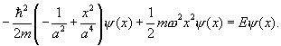
with the corresponding Schrödinger equation:
![]()
What will the solutions to this Schrödinger equation look like? Since the potential ½mw2 x2 increases without limit on going away from x = 0, no matter how much kinetic energy we give the particle, if it gets far enough from the origin the potential energy dominates, and the (bound state) wavefunction will decay increasing rapidly as x increases further. (Obviously, for a real physical oscillator there is a limit on the height of the potential—we will assume that limit is much greater than the energies in our problem.)
We know that when a particle penetrates a barrier of
constant height V0 (greater than the particle’s kinetic energy)
the wave function decreases exponentially into the barrier, as ![]() , where
, where ![]() . But, in contrast
to this constant height barrier, the “height” of the simple harmonic oscillator
potential continues to increase as the particle penetrates to larger x. Obviously, in this situation the decay will
be faster than exponential. If we
(rather naïvely) assume it is more or less locally exponential, but with
a local a varying with V0,
neglecting E relative V0 in the expression for a
suggests that a itself is
proportional to x, so maybe the wavefunction decays as
. But, in contrast
to this constant height barrier, the “height” of the simple harmonic oscillator
potential continues to increase as the particle penetrates to larger x. Obviously, in this situation the decay will
be faster than exponential. If we
(rather naïvely) assume it is more or less locally exponential, but with
a local a varying with V0,
neglecting E relative V0 in the expression for a
suggests that a itself is
proportional to x, so maybe the wavefunction decays as ![]() ?
?
To check this idea, we insert ![]() in the Schrödinger
equation, and use
in the Schrödinger
equation, and use
![]()
to find
![]()
The y(x) is just a factor here, and it is never zero, so can be cancelled out. This leaves a quadratic expression which must have the same coefficients of x0, x2 on the two sides, that is, the coefficient of x2 on the left hand side must be zero:
![]() .
.
This fixes the wave function. Equating the constant terms fixes the energy:
![]() .
.
So the conjectured form for the wave function is in fact the exact solution for the lowest energy state! (It’s the lowest state because it has no nodes.)
Also note that even in this ground state the energy is nonzero, just as it was for the square well. The central part of the wave function must have some curvature to join together the decreasing wave function on the left to that on the right. This “zero point energy” is sufficient in one physical case to melt the lattice—helium is liquid even down to absolute zero temperature (checked down to microkelvins!) because the wave function spread destabilizes the solid lattice that will form with sufficient external pressure.
Higher Energy States
It is clear from the above discussion of the ground state
that ![]() is the natural unit
of length in this problem, and
is the natural unit
of length in this problem, and ![]() that of energy, so to
investigate higher energy states we reformulate in dimensionless variables,
that of energy, so to
investigate higher energy states we reformulate in dimensionless variables,
![]() .
.
Schrödinger’s equation becomes
![]() .
.
Deep in the barrier, the e
term will become negligible, and just as for the ground state wave function,
higher bound state wave functions will be approximately of the form ![]() . (Of course, the equation itself will have the alternate
diverging solution
. (Of course, the equation itself will have the alternate
diverging solution ![]() except for special
values of the energy.)
except for special
values of the energy.)
The standard approach to solving the general problem is to
factor out the ![]() term,
term,
![]()
giving the differential equation for h(x):
![]()
We try solving this with a power series in x
: ![]() . Inserting this in the differential
equation, and requiring that the coefficient of each power x
n vanish identically, leads
to a recurrence formula for the coefficients hn:
. Inserting this in the differential
equation, and requiring that the coefficient of each power x
n vanish identically, leads
to a recurrence formula for the coefficients hn:
![]()
Evidently, the series of odd powers and that of even powers
are independent solutions to Schrödinger’s equation. For large n >>e,
the recurrence relation simplifies to ![]() . The series
therefore tends to
. The series
therefore tends to
![]() .
.
Multiply this by the ![]() factor to recover the
full wavefunction, we find it diverges as
factor to recover the
full wavefunction, we find it diverges as ![]() .
.
Actually we should have expected this—for a general value of
the energy, the Schrödinger equation has the solution ![]() at large distances,
and only at certain energies does the coefficient A vanish to give a
normalizable bound state wavefunction.
at large distances,
and only at certain energies does the coefficient A vanish to give a
normalizable bound state wavefunction.
So how do we find the nondiverging solutions? It is clear that the infinite power series must be stopped! The key is in the recurrence relation: if the energy satisfies 2e = 2n + 1, with n an integer, hn+2 and all higher coefficients vanish. The remaining nth order polynomial is called a Hermite polynomial and written Hn(x).
The standard normalization of the Hermite polynomials Hn(x) is to take the coefficient of the highest power xn to be 2n . The other coefficients are easy to find using the recurrence relation above, so:
![]()
So the bottom line is that the wavefunction for the nth
excited state, having energy ![]() , is
, is ![]() , where Cn is a normalization constant to
be determined in the next section.
, where Cn is a normalization constant to
be determined in the next section.
Differential Operator Approach to the Simple
Harmonic Oscillator
Actually, there is an easier way to find the energy levels of the quantum oscillator than the standard Schrödinger method given above. Continuing with the same dimensionless variables, we introduce the differential operators
![]()
These operators only have meaning if they are operating on a
function. It is crucial to note that if a product of these operators operates
on a function, the ![]() terms in each
operator also operate on any
terms in each
operator also operate on any ![]() ’s (in other operators) to their right. In particular, this
means that the two operators above do not commute, in fact
’s (in other operators) to their right. In particular, this
means that the two operators above do not commute, in fact
![]()
Schrödinger’s equation
![]()
can be written in terms of these differential operators:
![]()
Exercise: check that this is true.
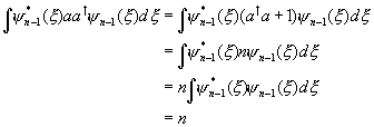
This leads to a surprisingly easy way to find all the solutions to the equation: suppose y(x) is a solution with energy e.
Multiplying the equation by ![]() ,
,
![]()
Now
![]()
![]()
Applying the operator gives the whole series of bound states, with energy increasing by one unit at each step, alternating between even and odd states. The operator a, on the other hand, goes down the ladder: operating on a state of energy e, it generates a state having energy e - 1. It must stop at the ground state, so that wave function is a solution of ay =0, or
![]()
This gives directly
![]()
for the ground state wavefunction, where we have added the normalization constant to give
![]() .
.
Note that the appropriately normalized solution in standard (not dimensionless) units is
![]()
The nth excited state, having energy (n + ½) in dimensionless units, is
![]() ,
,
where Cn is a normalization constant.
To find the normalization constant Cn ,
which is set by requiring by ![]() , we first observe that
, we first observe that ![]() .
.
Therefore
![]()
The last step can be established with an elementary
integration by parts (or in vector space notation by observing that ![]() is the adjoint of
is the adjoint of ![]() ).
).
The integral on the right is easily evaluated :
Therefore
![]() ,
,
taking the Cn’s real and positive.
In terms of the normalized wavefunctions yn(x), then, we have the important formula:
![]() .
.
Exercise: find the corresponding formula for a.
The final point in normalizing the bound state is to express
the function ![]() in terms of the nth order Hermite
polynomial. It is easy to check that
the coefficient of x n in
in terms of the nth order Hermite
polynomial. It is easy to check that
the coefficient of x n in ![]() is 2n/2,
and by definition that coefficient in the Hermite polynomial is 2n.
is 2n/2,
and by definition that coefficient in the Hermite polynomial is 2n.
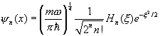
It follows that the correctly normalized (in x) wavefunction for the nth excited state is
Time Dependent States of the Simple Harmonic
Oscillator
Working with the time independent Schrödinger equation, as
we have in the above, implies that we are restricting ourselves to solutions of
the full Schrödinger equation which have a particularly simple time dependence,
an overall phase factor ![]() , and are states of definite energy E. However, the full time
dependent Schrödinger equation is a linear equation, so if y1(x,t)
and y2(x,t)
are solutions, so is any linear combination Ay1+By2.
Assuming y1
and y2
are definite energy solutions for different energies E1 and E2,
the combination will not correspond to a definite energy—a measurement of the
energy will give either E1
or E2, with appropriate
probabilities. This is still a
perfectly good, physically realizable wave function.
, and are states of definite energy E. However, the full time
dependent Schrödinger equation is a linear equation, so if y1(x,t)
and y2(x,t)
are solutions, so is any linear combination Ay1+By2.
Assuming y1
and y2
are definite energy solutions for different energies E1 and E2,
the combination will not correspond to a definite energy—a measurement of the
energy will give either E1
or E2, with appropriate
probabilities. This is still a
perfectly good, physically realizable wave function.
It is instructive to examine a combination state of this form a little more closely. We know that for the ground state wave function,
![]()
and for the first excited state,
![]() .
.
Suppose we simply add terms of this type together (neglecting the overall normalization constant for now), for example
![]() .
.
Looking at this wave function for t = 0, we notice that the two terms have the same sign for x > 0, and opposite signs for x < 0. Therefore, sketching the probability distribution for the
particle’s position, it is heavily skewed to the right (positive x).
However, the two terms have different time-dependent phases, differing
by a factor ![]() , so after time
, so after time ![]() has elapsed, a factor of -1 has evolved between the
terms. If we now look at the probability distribution |y|2,
it will be skewed to the left. In other
words, if the state is not of definite energy, the probability distribution can
vary in time. Of course, the total probability of finding the
particle somewhere stays the same.
Note that the probability distribution swings back and forth with the period of
the oscillator. This discussion also
implies that an ordinary pendulum, which clearly swings back and forth, cannot
be in a state of definite energy!
has elapsed, a factor of -1 has evolved between the
terms. If we now look at the probability distribution |y|2,
it will be skewed to the left. In other
words, if the state is not of definite energy, the probability distribution can
vary in time. Of course, the total probability of finding the
particle somewhere stays the same.
Note that the probability distribution swings back and forth with the period of
the oscillator. This discussion also
implies that an ordinary pendulum, which clearly swings back and forth, cannot
be in a state of definite energy!