Path Integrals in Quantum Mechanics
Michael Fowler
(Students please note: this is a draft version—I haven’t yet put in the diagrams I gave in class, but I hope this will still be useful.)
Huygen’s Picture of Wave Propagation
If a point source of light is switched on, the wavefront is an expanding sphere centered at the source. Huygens suggested that this could be understood if at any instant in time each point on the wavefront was regarded as a source of secondary wavelets, and the new wavefront a moment later was to be regarded as built up from the sum of these wavelets. For a light shining continuously, this process just keeps repeating.
What use is this idea? For one thing, it explains refraction—the change in direction of a wavefront on entering a different medium, such as a ray of light going from air into glass.
If the light moves more slowly in the glass, velocity v instead of c, with v < c, then Huygen’s picture explains Snell’s Law, that the ratio of the sines of the angles to the normal of incident and transmitted beams is constant, and in fact is the ratio c/v.
Fermat’s Principle of Least Time
We will now temporarily forget about the wave nature of light, and consider a narrow ray or beam of light shining from point A to point B, where we suppose A to be in air, B in glass. Fermat showed that the path of such a beam is given by the Principle of Least Time: a ray of light going from A to B by any other path would take longer. How can we see that? It’s obvious that any deviation from a straight line path in air or in the glass is going to add to the time taken, but what about moving slightly the point at which the beam enters the glass?
(Feynman gives a nice illustration: a lifeguard on a beach spots a swimmer in trouble some distance away, in a diagonal direction. He can run three times faster than he can swim. What is the quickest path to the swimmer?)
Moving the point of entry up a small distance d, the light has to travel an extra dsinq1 in air, but a distance less by dsinq2 in the glass, giving an extra travel time Dt = c/dsinq1- v/dsinq2. For the classical path, Snell’s Law gives sinq1/sinq2 = n = c/v, so Dt = 0 to first order. But if we look at a series of possible paths, each a small distance d away from the next at the point of crossing from air into glass, Dt becomes of order c/d away from the classical path.
Suppose now we imagine that the light actually travels along all these paths with about equal amplitude. What will be the total contribution of all these paths at B? Since the times along the paths are different, the signals along the different paths will arrive at B with different phases, and to get the total wave amplitude we must add a series of unit 2D vectors, one from each path. (Representing the amplitude and phase of the wave by a complex number for convenience—for a real wave, we can take the real part at the end.)
When we map out these unit 2D vectors, we find that in the neighborhood of the classical path, the phase varies little, but as we go away from it the phase spirals more and more rapidly, so those paths interfere amongst themselves destructively.
This is the explanation of Fermat’s Principle—only near the path of least time do paths stay approximately in phase with each other and add constructively. So this classical path rule has an underlying wave-phase explanation. In fact, the central role of phase in this analysis is sometimes emphasized by saying the light beam follows the path of stationary phase.
Classical Mechanics: The Principle of Least Action
Confining our attention for the moment to the mechanics of a single nonrelativistic particle in a potential, with Lagrangian L = T - V, the action S is defined by
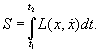
Newton’s Laws of Motion can be shown to be equivalent to the statement that a particle moving in the potential from A at t1 to B at t2 travels along the path that minimizes the action. This is called the Principle of Least Action: for example, the parabolic path followed by a ball thrown through the air minimizes the integral along the path of the action T-V where T is the ball’s kinetic energy, V its gravitational potential energy (neglecting air resistance, of course).
With the advent of quantum mechanics, and the realization that any particle, including a thrown ball, has wave like properties, the rather mysterious Principle of Least Action looks a lot like Fermat’s Principle of Least Time. Recall that Fermat’s Principle works because the total phase along a path is the integrated time elapsed along the path, and for a path where that integral is stationary for small path variations, neighboring paths add constructively, and no other sets of paths do. If the Principle of Least Action has a similar explanation, then the wave amplitude for a particle going along a path from A to B must have a phase equal to some constant times the action along that path. If this is the case, then the observed path followed will be just that of least action, for only near that path will the amplitudes add constructively, just as in Fermat’s analysis of light rays.
Going from Classical Mechanics to Quantum Mechanics
Of course, if we write a phase factor for a path eicS where S is the action for the path
and c is some constant, c must necessarily have the dimensions of
inverse action. Fortunately, there is a natural candidate for the constant c. The wave nature of matter arises from
quantum mechanics, and the fundamental constant of quantum mechanics, Planck’s
constant, is in fact a unit of action. It turns out that the appropriate path
phase factor is ![]() .
.
That the phase factor is ![]() , rather than
, rather than ![]() , say, can be established by considering the double slit
experiment for electrons (Peskin page 277).
Suppose electrons from the top slit, Path I, go a distance D to
the detector, those from the bottom slit, Path II, go D + d, with
d << D. Then if the electrons have wavelength l we
know the phase difference at the detector is 2pd/l. To see this from our formula for summing
over paths, on Path I the action S
= Et = ½mv12t, and v1
= D/t, so
, say, can be established by considering the double slit
experiment for electrons (Peskin page 277).
Suppose electrons from the top slit, Path I, go a distance D to
the detector, those from the bottom slit, Path II, go D + d, with
d << D. Then if the electrons have wavelength l we
know the phase difference at the detector is 2pd/l. To see this from our formula for summing
over paths, on Path I the action S
= Et = ½mv12t, and v1
= D/t, so
S1 = ½mD2/t.
For Path II, we must take v2 = (D + d)/t. Keeping only terms of leading order in d/D, the action difference between the two paths
S2 - S1 = mDd/t
So the phase difference
![]()
This is the known correct result, and this fixes the constant multiplying the action/h in the expression for the path phase.
In quantum mechanics, such as the motion of an electron in an atom, we know that the particle does not follow a well-defined path, in contrast to classical mechanics. Where does the crossover to a well-defined path take place? Taking the simplest possible case of a free particle (no potential) of mass m moving at speed v, the action along a straight line path taking time t from A to B is ½mv2t. If this action is of order Planck’s constant h, then the phase factor will not oscillate violently on moving to different paths, and a range of paths will contribute. In other words, quantum rather than classical behavior dominates when ½mv2t is of order h. But vt is the path length L, and mv/h is the wavelength l, so we conclude that we must use quantum mechanics when the wavelength h/p is significant compared with the path length. Interference sets in when the difference in path actions is of order h, so in the atomic regime many paths must be included.
Feynman (in Feynman and Hibbs) gives a nice picture to help think about summing over paths. He begins with the double slit experiment for an electron. We suppose the electron is emitted from some source A on the left, and we look for it at a point B on a screen to the right. In the middle is a thin opaque barrier with the familiar two slits. Evidently, to find the amplitude for the electron to reach B we sum over two paths. Now suppose we add another two-slit barrier. We have to sum over four paths. Now add another. Next, replace the two slits in each barrier by several slits. We must sum over a multitude of paths! Finally, increase the number of barriers to some large number N, and at the same time increase the number of slits to the point that there are no barriers left. We are left with a sum over all possible paths through space from A to B, multiplying each path by the appropriate action phase factor.
In fact, the sum over paths is even more daunting than this picture suggests. All the paths going through these many slitted barriers are progressing in a forward direction, from A towards B. Actually, if we’re summing over all paths, we should be including the possibility of paths zigzagging backwards and forwards as well, eventually arriving at B. We shall soon see how to deal systematically with all possible paths.
Propagation of a Free Electron from A to B.
As a warm up exercise, we consider an electron confined to one dimension, with no potential present, moving from x¢ at time t¢ to x at time t. This is a problem easily solved by the standard quantum mechanical techniques introduced last semester, so we do that first then go on to see how the same solution emerges in a sum over all possible paths.
Recall that we introduced the propagator U(x,t; x¢, t¢), the probability amplitude for an electron to be at x at time t given that it was at x¢ at time t¢. This is exactly what we are trying to find. It is defined by:
![]()
where x¢ is to be regarded as a dummy variable, that is, it is integrated over. For t-t¢ = 0, the propagator reduces, as it must, to the identity operator.
The set of states summed over is the set of eigenstates of the Hamiltonian, for the one-dimensional free particle this is just the set of plane wave states, so
![]()
This is a standard Gaussian integral, recall
![]()
Taking t¢ = 0 for convenience, we find
![]()
Now let us think about the sum over paths. Following Shankar (page 226) let us assume that the classical path dominates, and that only paths in its neighborhood contribute, and all the other paths do is multiply the effect of the single classical path by some constant. The classical path, of course, corresponds to motion from x¢ to x at a constant speed v = (x - x¢)/t. The action along this path is therefore Et, where E is the classical energy ½ mv2 , giving
![]()
This gives the correct exponential term. The prefactor A¢ can be determined from the requirement that as t goes to zero, U must approach a delta function. From one definition of the delta function,
![]()
we find that A¢ must in fact exactly match the prefactor found above by conventional means. However, we have been lucky—in more interesting situations, the classical path doesn’t give all the information, and we really must address the issue of integrating over all paths.
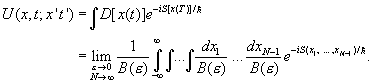
Integrating Over Paths
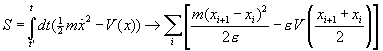
We begin with a particle in one dimension going from x¢ at time t¢ to x at time t. We enumerate the paths in a crude way, reminiscent of Riemann integration. We divide the time interval t¢ to t into N equal intervals each of duration e, so t¢ = t0, t1 = t0 + e, t2 = t0 + 2e, … t = tN. We then define a particular path from x to x¢ by specifying the position of the particle at each of the intermediate times, that is, it is at x1 at time t1, x2 at time t2 and so on. Then we simplify the path by putting in straight line bits between x0 and x1, x1 and x2, etc. The justification is that when we take the limit of e going to zero, this will become a true representation of the path.
The next step is to sum over all possible paths with a
factor ![]() for each one. The sum
is accomplished by integrating over all possible values of the intermediate
positions x1, x2, … xN-1
and then taking N to infinity.
for each one. The sum
is accomplished by integrating over all possible values of the intermediate
positions x1, x2, … xN-1
and then taking N to infinity.
The action on the zigzag path is
We define the “integral over paths” written ![]() by
by
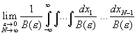
where we haven’t yet figured out what the overall weighting factor B(e) is going to be.
To summarize: the propagator U(x,t;
x¢,
t¢)
is the amplitude for a particle localized at x¢ at time t¢ to
be found at x at time t.
In terms of the eigenstates |x> of the position
operator, the particle is initially in state |x¢>. This is not, of
course, an eigenstate of the Hamiltonian, and after time t-t¢ it
has evolved to the state ![]() . Therefore,
. Therefore, ![]() and this is precisely the Schrödinger wavefunction y(x,t)
of a particle localized at x¢ at earlier time t¢, with Hamiltonian H. Consequently, U(x,t; x¢, t¢)
regarded as a function of x, t satisfies Schrödinger’s equation
and this is precisely the Schrödinger wavefunction y(x,t)
of a particle localized at x¢ at earlier time t¢, with Hamiltonian H. Consequently, U(x,t; x¢, t¢)
regarded as a function of x, t satisfies Schrödinger’s equation
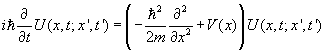
We are claiming that this same U(x,t; x¢, t¢) is given by:
We shall establish this equivalence by proving that it satisfies the same differential equation. It clearly has the same initial value—as t¢ and t coincide, it goes to d(x - x¢) in both representations.
To differentiate ![]() with respect to t, we isolate the integral over the
last path variable, xN-1:
with respect to t, we isolate the integral over the
last path variable, xN-1:
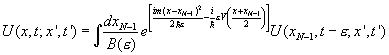
Now in the limit e going to zero, almost all
the contribution to this integral must come from close to the point of
stationary phase, that is, xN-1 = x.
In that limit, we can take ![]() to be a slowly varying function of xN-1, and replace it by the leading terms in a
Taylor expansion about x, so
to be a slowly varying function of xN-1, and replace it by the leading terms in a
Taylor expansion about x, so
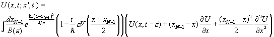
The xN-1 dependence in the potential V can be neglected in leading order—that leaves standard Gaussian integrals, and
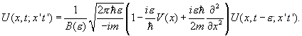
Taking the limit of e going to zero fixes our unknown normalizing factor,
![]()
giving
 .
.