Saddlepoint Methods in Contour Integration
Michael
Fowler
Analytic Functions
Suppose we have a complex function f = u + iv of a complex variable z = x + iy, defined in some region of the complex plane, where u, v, x, y are real. That is to say,
![]()
with u(x,y) and v(x,y) real functions in the plane.
We now assert that in this region f(z) is differentiable, that is to say,
![]()
is well-defined. What does this tell us about the functions u(x,y) and v(x,y), the real and imaginary parts of f(z)?
In fact, the property of differentiability for a function of a complex variable tells us a lot! It does not just mean that the function is reasonably smooth. The crucial difference from a function of a real variable is that D z can approach zero from any direction in the complex plane, and the limit in these different directions must be the same. Of course, there are only two independent directions, so what we are really saying is
![]()
which we can write in terms of u,v:
![]()
Equating real and imaginary parts of this equation we find:
![]()
These are called the Cauchy-Riemann equations.
It immediately follows that both u(x,y) and v(x,y) must satisfy the two-dimensional Laplacian equation,
![]()
Notice that this implies (just as for an electrostatic potential) that u(x,y) cannot have an absolute minimum or maximum inside the region of analyticity. If df(z)/dz = 0, but the second-order partial derivatives are nonzero, then they must have opposite sign, signaling a saddlepoint. In the general case, a two-dimensional version of Gauss’ theorem can be used to show there is no local extremum.
Furthermore,
![]()
That is to say, the contour lines of constant u(x,y) are everywhere orthogonal to the contour lines of constant v(x,y). (The gradient being orthogonal to the contour lines everywhere.)
The important point is that just requiring differentiability of a function of a complex variable imposes a strong constraint on its real and imaginary parts, the functions u(x,y) and v(x,y).
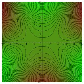
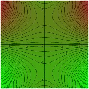
A Simple Example: f (z) = z 2.
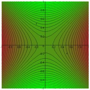
It is worthwhile building a clear picture of the real and imaginary parts of the function z2. The real part is x2 - y2, and its contour lines in the square -1 to 1 are shown below. We have chosen geographic coloring: green for valleys, brown for hills. At the origin, there is a saddlepoint with higher ground in both directions of the real axis, lower ground in the pure imaginary directions. The lines x = y, x = -y (not shown) are contours at the same level (zero) as the origin.
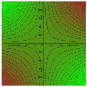
What about the imaginary part? Imz2 = 2xy has contours:
Putting the two sets of contour lines on the same diagram it is clear that they always cut each other orthogonally:
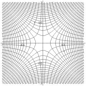
(Incidentally, this picture has a physical realization. It represents the field lines and equipotentials of a quadrupole magnet, used for focusing beams of charged particles.)
Saddlepoints of Analytic Functions
Suppose we have a function f(z) analytic in some region R of the complex plane, and at some point z0 inside R the derivative df(z)/dz = 0. Then in the neighborhood of z0,
![]()
Close enough to z0 we can neglect the higher order terms, and for the case of f ¢¢(z0) real, the contour lines of the real and imaginary parts of f(z) will then be exactly those we have plotted for z2 above. For f ¢¢(z0) complex, the plots will be rotated by an angle equal to the phase of f ¢¢(z0).
That is to say, for any analytic function, near any point where df(z)/dz = 0, the real and imaginary parts of the function have saddlepoints with contour maps rotated versions of those above.
Integrating Through a Saddlepoint
We consider now integrals of the form
![]()
where C is some path in a region where f(z) is analytic. This means the value of the integral will not be affected by distorting the path, provided it stays in the region of analyticity. (The path of integration is usually called the contour of integration—we’ll call it path here, to avoid confusion with our contours, which have the standard geographic meaning, joining points having the same value of some parameter.)
Note that with the exponential form of the integrand, the real part of f(z) determines the magnitude of the integrand, the imaginary part of f(z) determines its phase.
The strategy is to arrange the path of integration so that as much as possible of it is in the valleys, where the integrand is small, then to go over the saddlepoint by the steepest possible route, which would be staying on the imaginary axis in the case of z2 plotted above. It is important to note that this “steepest descent” route is also a path along which the imaginary part of f(z) remains constant, so the contributions along this path are all in phase, that is to say, they add coherently.
The bottom line is that by directing the path of integration through the saddlepoint along the steepest route for the magnitude of the integrand, the biggest contributions to the integral are all in phase. Along this path, the integral has standard Gaussian form. If the function f(z) is sufficiently large, it may be that the contribution of the integral away from the saddlepoint can be neglected. This method is therefore often valuable in cases where some parameter becomes large: we give a number of examples to clarify this point.
Saddlepoint Estimation of n!
We use the identity
![]()
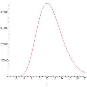
To picture tne-t, here it is for n = 10:
Note that
Therefore, in the neighborhood of the maximum value of f(t) at t = n,
![]()
For integer n, the function is analytic in any finite region of the complex plane. Taking n = 10, as in the real-axis graph above, and plotting the contours of Re(tne-t) in the neighborhood of t = 10, we find:
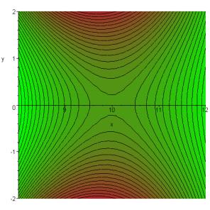
It is clear that the integral along the real axis is in fact a steepest descent path. The reason we look at this straightforward case is to gain some experience about when it is reasonable to throw away all the contribution to the integral except that near the saddlepoint. If we simply take
![]()
and take the t integration to be over the whole real axis, not just positive t, it is a Gaussian integral and
![]()
More precise, and considerably more complicated, methods give the leading correction to this expression. It is down by a factor of 1/12n, so the naïve Gaussian saddlepoint result is accurate within 1% for n = 10, and improves as n increases.
The Delta Function
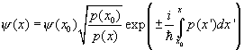
Recall that the delta function can be defined by the limit of a Gaussian integral
![]() .
.
It is easy to see how this leads to
![]()
for an integral along the real axis with a function f(x) reasonably well-behaved near the origin. Shankar mentions that the definition also works even if D2 is replaced by iD2. In that case, the absolute value of the function is the same everywhere on the real axis, and increases as D-1 on taking D small. The reason it still works is that the phase oscillations are so rapid everywhere except at the origin, where the phase is momentarily stationary, so all the contribution comes from there.
However, it is easier to believe
![]()
on going into the complex plane. If we change variables from x to x, where x2 = ix 2, the integral again becomes a simple real Gaussian. But, regarding x as a complex variable, transforming to x is just equivalent to rotating the axes by p/4, or multiplying by the square root of i. The steepest descent route through the origin is now along the line at p/4 to the real axis. So this is a perfectly good definition of the d-function provided we can distort the path of integration from the real axis to the line x = y. (Strictly speaking, the path would now include two octants of a circle at very large R—their contribution vanishes in the limit of R going to infinity.)
WKB Connection Formulas
The WKB semiclassical approximate solution to Schrödinger’s equation,
is reliable in regions where the wavelength (for oscillating solutions) or the decay length (for exponential solutions) changes only slightly over a distance of one wavelength or decay length respectively. For a particle trapped in a (one-dimensional) potential well, classically the particle would bounce back and forth between the two turning points where its kinetic energy vanishes. In the quantum case, these are precisely the points where the wavelength becomes infinite, so the WKB solution fails.
However, for a reasonably smooth potential it may be an adequate approximation to treat a turning point region as one where the potential is increasing linearly with distance over a sufficient range that beyond this point the WKB approximation can be used in both directions.
The solution of Schrödinger’s equation for a linearly increasing or decreasing potential is well known, it is the Airy function, the solution of the differential equation
![]()
plotted here at the left-hand turning point :
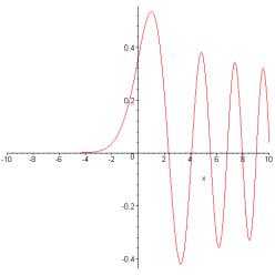
The strategy is to evaluate this function for large x, both positive and negative, so that we can join together the two WKB solutions, valid in the far regions, in a quantitative fashion.
Following Mathews and Walker (page 116) the differential equation is most simply solved by taking its Fourier transform.
If
![]()
then
![]()
Therefore
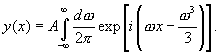
This is an exact result, but a nontrivial integral! Fortunately, we are only interested in its value for large values of |x|, and this is precisely where saddlepoint methods become accurate.
To see where the saddlepoints are, and how they relate to an integral along the real axis, we plot contour maps of the term in the exponential.
Large positive x:
In the map below, we take x = 10 (rather small), so the
saddlepoints are at ![]() . If the real axis
path of integration is moved down into the (green) valleys, the contour can come
up towards the left saddlepoint from the bottom left, over the saddle into the
top center valley, then back over the second saddlepoint into the bottom right
valley and on the infinity.
. If the real axis
path of integration is moved down into the (green) valleys, the contour can come
up towards the left saddlepoint from the bottom left, over the saddle into the
top center valley, then back over the second saddlepoint into the bottom right
valley and on the infinity.
Writing the integral as
![]()
(dropping irrelevant overall constants) then
(Mathews and Walker take the “large” parameter x out of f, we’ve left it in—this doesn’t affect the final result.)
Near the positive saddlepoint
![]()
dropping higher-order terms. Since f ¢¢ is pure imaginary at the saddlepoint, the appropriate path for a real exponent in the Gaussian integral is at p/4 to the x-axis. So in the path integral
![]()
where ds is a real parameter measuring incremental path length, and the sign in the exponent is positive for the saddlepoint on the left. The contributions from the two saddlepoints give the asymptotic (large positive x) solutions as:
![]()
Large negative x: In this case, the saddlepoint geography is quite different, although the distant geography is the same, being dominated by the w 3 term.
Just as before, the real axis integration path can be moved down from the real axis into the valleys at bottom left and bottom right. (The extra contributions from linking up the new path with the real axis at infinity are zero.) It is clear from the map above that to get from the valley on the left to the one on the right means just going over the saddlepoint on the negative imaginary axis. Note from the darker shading that the other saddlepoint is at higher elevation.
The integration through the saddlepoint is parallel to the real axis, and gives
![]()
This, then, is the decaying wavefunction solution of the Airy equation that we are looking for, and it is clear that it goes smoothly from the exponential to the cosine form as x is taken along the real axis from large negative to large positive values.