Evaluating Rapidly Oscillating Integrals by Steepest Descents

How to evaluate in an unambiguous fashion: an introduction to moving the contour of integration and the Method of Steepest Descent.

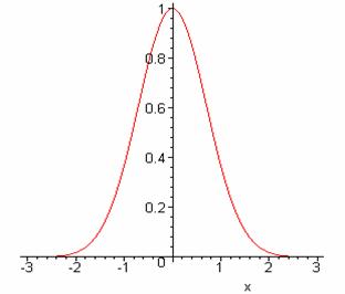
The familiar Gaussian integral is easy to understand. Plotting the integrand, (here for a = 1) there is a peak of height 1 and width of order 1/Öa.

But what about the result ? This (correct) result is far less obvious! Here the integrand is always on the unit circle in the complex plane, and equal to 1 at x = 0. It is instructive to plot the phase of the integrand as a function of x (taking a = 1 in the graph below).

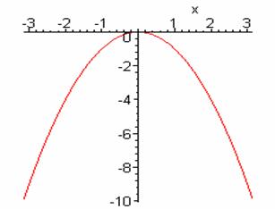
The phase is stationary at the origin, so contributions from that region add coherently. To help visualize the integrand better, here’s a plot of the real part:

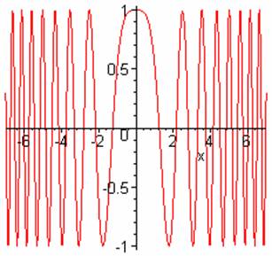
It is evident that almost all the contribution to the integral comes from the central region where the phase is stationary, the increasingly rapid oscillations away from the origin ensuring that very little comes from elsewhere.

So how do we actually evaluate the integral? In the complex plane z = x + iy, we can write

Notice that the amplitude of the integrand on the real axis, so it does not go to zero at infinity, although there are essentially no contributions from large x because of the rapid oscillations.

A cleaner way to see what’s going on is to rotate the contour of integration around the origin to the 45 degree line x = -y. It’s safe to do this because the amplitude of the integrand decreases on going from the real axis into the region xy < 0, and in fact tends to zero on going to infinity in that region.

y

	y

The integral becomes with so

the required result.

Steepest Descent Method

In fact, the contour rotation trick used above to make the integral easier to evaluate is a particular case of a method having wide applicability in evaluating contour integrals of the form . The basic strategy is to distort the contour of integration in the complex z-plane so that the amplitude of the integrand is as small as possible over as much of the contour of integration as possible. Actually, that is exactly what we did in the example above. To see this, it is helpful to plot the contour lines (lines of constant value) of the modulus of the integrand,

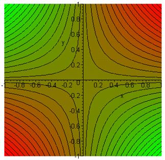
The convention here is red for the high ground, green for the valleys. We want to keep the contour of integration as low as possible for as long as possible. The map above is of a “saddlepoint”: hills rise to the northeast and the southwest of the origin, valleys fall away to the northwest and the southeast. The strategy is to stay in the valleys (small integrand) as much as possible—however, to get from -¥ to +¥ we have to get from one valley to the other, and that means going over the saddlepoint at the origin. Obviously, to get the integrand as small as possible at all stages in the integration we must go down from the saddlepoint in both directions by the steepest possible route, and it is evident that this is right down the center of the valley, just the contour we chose above.

Note that this steepest descent path is also one of stationary phase. This is because for any analytic function of a complex variable f(z), the lines of constant Ref(z) are perpendicular to those of constant Imf(z). For a function , the steepest descent line is perpendicular to the lines of constant Ref(z), and is therefore a line of constant Imf(z), that is, constant phase of .