previous index next PDF
Schrödinger’s Equation in 1-D: Some Examples
Michael Fowler,
UVa. 9/24/07
Curvature of Wave Functions
Schrödinger’s equation in the form
![]()
can be interpreted by saying that the left-hand side, the
rate of change of slope, is the curvature
– so the curvature of the function is proportional to ![]() This means that if E
> V(x), for
This means that if E
> V(x), for ![]() positive
positive ![]() is curving negatively, for
is curving negatively, for ![]() negative
negative ![]() is curving positively.
In both cases,
is curving positively.
In both cases,![]() is always curving towards the x-axis—so, for E
> V(x),
is always curving towards the x-axis—so, for E
> V(x), ![]() has a kind of
stability: its curvature is always bringing it back towards the axis, and so
generating oscillations. The simplest example
is that of a constant potential V(x)
= V0 < E, for which the wave function is
has a kind of
stability: its curvature is always bringing it back towards the axis, and so
generating oscillations. The simplest example
is that of a constant potential V(x)
= V0 < E, for which the wave function is ![]() with
with ![]() a constant and
a constant and ![]()
On the other hand, for V(x) > E, the curvature is always away
from the axis. This means that ![]() tends to diverge to
infinity. Only with exactly the right
initial conditions will the curvature be just right to bring the wave function
to zero as x goes to infinity. (This
is possible because as
tends to diverge to
infinity. Only with exactly the right
initial conditions will the curvature be just right to bring the wave function
to zero as x goes to infinity. (This
is possible because as ![]() tends to zero, the
curvature tends to zero, too.)
tends to zero, the
curvature tends to zero, too.)
For a constant potential V0
> E, the wave function is ![]() , with
, with ![]() Of course, this wave
function will diverge in at least one direction! However, as we shall see below, there are
situations with spatially varying potentials where this wave function is only
relevant for positive x, and the
coefficients A, B are functions of the energy—for certain energies it turns out
that
Of course, this wave
function will diverge in at least one direction! However, as we shall see below, there are
situations with spatially varying potentials where this wave function is only
relevant for positive x, and the
coefficients A, B are functions of the energy—for certain energies it turns out
that ![]() , and the wave function converges.
, and the wave function converges.
One Dimensional Infinite Depth Square Well
In an earlier lecture, we considered in some detail the
allowed wave functions and energies for a particle trapped in an infinitely
deep square well, that is, between infinitely high walls a distance L apart.
For that case, the potential between the walls is identically zero so
the wave function has the form ![]() The wave function
The wave function![]() necessarily goes to zero right at the walls, since it cannot
have a discontinuity, and must be zero just inside the wall. Even a quantum particle cannot penetrate an
infinite wall!
necessarily goes to zero right at the walls, since it cannot
have a discontinuity, and must be zero just inside the wall. Even a quantum particle cannot penetrate an
infinite wall!
An immediate consequence is that the lowest state cannot
have zero energy, since k = 0 gives a
constant ![]() . Rather, the lowest
energy state must have the minimal amount of bending of the wave function
necessary for it to be zero at both
walls but nonzero in between—this corresponds to half a period of a sine or
cosine (depending on the choice of origin), these functions being the solutions
of Schrödinger’s equation in the zero potential region between the walls. The allowed wave functions (eigenstates)
found as the energy increases have successively
0, 1, 2, … zeros (nodes) in the well.
. Rather, the lowest
energy state must have the minimal amount of bending of the wave function
necessary for it to be zero at both
walls but nonzero in between—this corresponds to half a period of a sine or
cosine (depending on the choice of origin), these functions being the solutions
of Schrödinger’s equation in the zero potential region between the walls. The allowed wave functions (eigenstates)
found as the energy increases have successively
0, 1, 2, … zeros (nodes) in the well.
Parity of a Wave Function
Notice that the allowed wave eigenfunctions of the
Hamiltonian for the infinite well are symmetrical or antisymmetrical about the
center, ![]()
We call the operator that reflects a function in the origin
the parity operator P, so
these eigenstates of the Hamiltonian are also
eigenstates of the parity operator, with eigenvalues ±1. This is
because the Hamiltonian is itself symmetric: ![]() is even in x,
and so is V(x), so
is even in x,
and so is V(x), so ![]() , and the two operators can be simultaneously diagonalized,
that is, a common set of eigenstates can be constructed.
, and the two operators can be simultaneously diagonalized,
that is, a common set of eigenstates can be constructed.
Finite Depth Square
If the potential at the walls is not infinite, the parity
operator P will continue to commute
with the Hamiltonian H as long as the
potential is symmetric, ![]() .
.
We take
V(x) = V0 for x < -L/2
V(x) = 0 for -L/2 < x < L/2
V(x) = V0 for L/2 < x.
We only need look for solutions symmetric or antisymmetric
about the origin. This is important from
a practical point of view, because it allows us to integrate Schrödinger’s
equation numerically out from the origin in the positive direction: ![]() in the negative
direction is fixed by symmetry (or antisymmetry). Since it’s a second-order equation, we need
two boundary conditions to get going, for symmetric states, we can take
in the negative
direction is fixed by symmetry (or antisymmetry). Since it’s a second-order equation, we need
two boundary conditions to get going, for symmetric states, we can take ![]() for antisymmetric states,
for antisymmetric states, ![]() (Of course, we will
have to normalize
(Of course, we will
have to normalize ![]() correctly eventually.)
correctly eventually.)
The numerical strategy is to pick a value for the energy E, choose one of the boundary conditions
above and integrate ![]() numerically to a large
positive value of x. For almost all values of E, the wave function will be exponentially increasing with x.
For the particular values corresponding to bound states, it will be
exponentially decreasing.
numerically to a large
positive value of x. For almost all values of E, the wave function will be exponentially increasing with x.
For the particular values corresponding to bound states, it will be
exponentially decreasing.
It is well worth while building up an intuition for this by playing with the spreadsheet accompanying this lecture: the spreadsheet does the numerical integration for any E and well depth, and has a macro to locate the nearest bound state.
Joining the Wave Functions Inside and Outside of the Well
The numerical method mentioned above works for any symmetric potential. Fortunately, for the square well, an analytic/graphical method is very effective, and provides more insight.
Let us begin by considering how the lowest energy state wave
function is affected by having finite instead of infinite walls. Inside the well, where V = 0, the solution to Schrödinger’s equation is still of cosine
form (for a symmetric state). However, Schrödinger’s equation now has a nonzero
solution inside the wall ![]() , where
, where ![]() :
:
![]() ,
,
has two exponential solutions one increasing with x, the other decreasing,
![]() .
.
We are assuming here that E < V0, so the particle is bound to the well. We shall find the lowest energy state is always bound in a finite square well, however weak the potential.
Now, Schrödinger’s equation must be valid everywhere,
including the point ![]() . Since the potential is finite, the wave function
. Since the potential is finite, the wave function ![]() and its first derivative must be continuous at x = L/2.
and its first derivative must be continuous at x = L/2.
Suppose, then, we choose a particular energy E. Then the wavefunction inside the well
(taking the symmetric case) is proportional to coskx, where ![]() . The wave function (and its derivative!) must match a
sum of exponential terms at x = L/2, so
. The wave function (and its derivative!) must match a
sum of exponential terms at x = L/2, so

Solving these equations for the coefficients A, B in the usual way, we find that in general the cosine solution inside the well goes smoothly into a linear combination of exponentially increasing and decreasing terms in the wall. However, this cannot in general represent a bound state in the well. The increasing solution increases without limit as x goes to infinity, so since the square of the wave function is proportional to the probability of finding the particle at any point, the particle is infinitely more likely to be found at infinity than anywhere else. It got away! This clearly makes no sense – we’re trying to find wave functions for particles that stay in, or at least close to, the well. We are forced to conclude that the only exponential wave function that makes sense is the one for which A is exactly zero, so that there is only a decreasing wave in the wall.
Finding the Bound
State
If we demand that the wavefunction decrease exponentially as x goes to infinity, or, in other words, require A to be zero, k must satisfy the condition given be dividing one of the boundary equations above by the other:
![]() .
.
This equation cannot be solved analytically, but is easy to
solve graphically by plotting the two sides as functions of k (recall ![]() , and
, and ![]() ) and finding where the curves intersect.
) and finding where the curves intersect.
From
![]()
note that this is real only for
![]()
(Because if this inequality is not satisfied, the particle has enough kinetic energy to get out of the well!)
Now the condition for a bound state can be written
![]()
Cleaning up the appearance of the equation by choosing
variables ![]() and plotting
and plotting from x = 0 to x = a, allowed bound
state k-values correspond to the
points of intersection of the two curves.
The bound state energies are then given by
from x = 0 to x = a, allowed bound
state k-values correspond to the
points of intersection of the two curves.
The bound state energies are then given by ![]()
The variable a is a measure of the attractive strength of the well. Here are the two curves for a shallow well (a = 1):
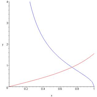
It
is interesting to note that however small a is, the curve  goes to infinity as x
goes to zero, so will always intersect y
= tanx: there will always be a bound state.
goes to infinity as x
goes to zero, so will always intersect y
= tanx: there will always be a bound state.
A deeper well, a = 20, gives several bound states:
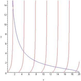
For the lower energies at least, the allowed k–values are approximately linearly spaced, at about π/2, 3π/2, 5π/2, … so the bound state energies are not far off the 1, 9, 25,… pattern of the infinitely deep square well—remembering that we are only looking at the even parity (cosine) solutions!
Exercise: Use
the spreadsheet with D
= 50, W = 4 and find all the even
bound state energies. How well do they
fit this pattern? Can you account for
the deviation? Examine the wave functions for the different eigenenergies: note
how far it penetrates the wall, and how much that changes the boundary
condition at the wall from that for an infinite wall. Which one of the bound
state energies is most affected by this, and how is it affected? Would you
expect that from the graphical solution?
The odd parity solutions, sine waves inside the well, can be found by an exactly similar analysis. One difference is that an arbitrarily weak well will not bind an odd parity state. The point is that for a weak potential to bind an even state, it only has to curve the wave function slightly to get from one exponentially decaying to the left to one exponentially decaying to the right. These curves decay very slowly for a weak potential, and give a bound state in which the particle is most likely to be found outside the well. On the other hand, in an odd solution the wave function within the well has to have enough total curvature to fit together two decaying wave functions which have opposite sign. This takes much more bending, and cannot be achieved with a very weak potential.
Exercise: Check this last statement, by considering what fraction of a wavelength of the oscillating wave function inside the well is necessary to make a connection between the decaying wave functions in the walls to the left and right.
The Delta Function Potential
One limiting case of a square well is a very narrow deep well, which can be approximated by a delta function when the range of variation of the wave function is much greater than the range of the potential, so Schrödinger’s equation becomes
![]()
with ![]() negative for an
attractive potential.
negative for an
attractive potential.
The infinity of the ![]() -function cannot be balanced by the finite right hand side,
so the wave function must have a discontinuity in slope at the origin.
-function cannot be balanced by the finite right hand side,
so the wave function must have a discontinuity in slope at the origin.
To find the ground state energy, note first that as a
one-dimensional attractive potential there will be a bound state: any change in
slope is sufficient to connect an exponentially increasing function coming in
from ![]() to a decreasing one
going to
to a decreasing one
going to ![]() since the rates of
increase and decrease can be arbitrarily slow.
since the rates of
increase and decrease can be arbitrarily slow.
Away from the origin, then, we can take the wave function to be
![]() ,
,
the energy of the state being ![]() .
.
The discontinuity in slope at the origin is just
![]() .
.
To match this with the ![]() -function singularity, we integrate the Schrödinger equation
term by term from
-function singularity, we integrate the Schrödinger equation
term by term from ![]() to
to ![]() in the limit of
in the limit of ![]() going to zero:
going to zero:
![]()
Note first that the right-hand side, having a finite
integrand, must go to zero in the limit of ![]() going to zero.
going to zero.
The ![]() -function term must integrate to
-function term must integrate to ![]()
The first term just gives the discontinuity in slope,
Schrödinger’s equation is therefore satisfied if ![]() (remembering
(remembering ![]() is negative for an
attractive potential).
is negative for an
attractive potential).
The energy of the bound state is
![]()
Exercise: rederive this result by taking the limit
of a narrow deep well, tending to a ![]() -function, with a cosine wave function inside.
-function, with a cosine wave function inside.
A Potential Step
Our analysis so far has been limited to real-valued
solutions of the time-independent Schrödinger equation. This is fine for analyzing bound states in a
potential, or standing waves in general, but cannot be used, for example, to
represent an electron traveling through space after being emitted by an electron
gun, such as in a TV tube. The reason is
that a real-valued wave function ![]() , in an energetically allowed region, is made up of terms
locally like coskx and sinkx, multiplied in the full wave function
by the time dependent phase factor
, in an energetically allowed region, is made up of terms
locally like coskx and sinkx, multiplied in the full wave function
by the time dependent phase factor ![]() , giving equal amplitudes of right moving waves
, giving equal amplitudes of right moving waves ![]() and left moving waves
and left moving waves ![]() . So, for an electron
definitely moving to the right, even the time-independent part of the wave
function must necessarily be complex.
. So, for an electron
definitely moving to the right, even the time-independent part of the wave
function must necessarily be complex.
Consider an electron of energy E moving in one dimension through a region of zero potential from large negative x and encountering an upward step potential of height V0 (V0 < E) at the origin x = 0. Of course, strictly speaking, the electron should be represented by a wave packet, and hence could not have a precisely defined energy E, but we assume here that it is a very long wave packet, very close to a plane wave, so we take it that the wave function is:
![]() for x < 0
for x < 0
(A more precise analysis, in which an incoming wave packet is used, can be done by solving for the plane-wave components individually. In the limit of a wavepacket long compared to the de Broglie wavelength, the result is the same as that found here.)
Visualizing the classical picture of a particle approaching a hill (smoothing off the corners a bit) that it definitely has enough energy to surmount, we would perhaps expect that the wave function continues beyond x = 0 in the form
![]() for x > 0,
for x > 0,
where k1 corresponds to the slower speed the particle will have after climbing the hill.
Schrödinger’s equation requires that the wave function have no discontinuities and no kinks (discontinuities in slope) so the x < 0 and x > 0 wave functions must match smoothly at the origin. For them to have the same value, we see from above that A = B. For them to have the same slope we must have kA = k1B. Unfortunately, the only way to satisfy both these equations with our above wave functions is to take k = k1—which means there is no step potential at all!
Question: what is wrong with the above reasoning?
The answer is that we have been led astray by the depiction of the particles as little balls rolling along in a potential, with enough energy to get up the hill, etc. Schrödinger’s equation is a wave equation. Building intuition about solutions should rely on experience with waves. We should be thinking about a light wave going from air into glass, for example. If we do, we realize that at any interface some of the light gets reflected. This means that our expression for the wave function for x < 0 is incomplete, we need to add a reflected wave, giving
![]() for x < 0
for x < 0
![]() for x
> 0.
for x
> 0.
Now matching the wave function and its derivative at the origin,
![]()
The fraction of the wave that is reflected

Evidently, the fraction of the wave transmitted
![]() .
.
Question: isn’t the amount transmitted just given by B2/A2?
The answer is no. The ratio B2/A2 gives the relative probability of finding a particle in some small region in the transmitted stream relative to that in the incoming stream, but the particles in the transmitted stream are moving more slowly, by a factor k1/k. That means that just comparing the densities of particles in the transmitted and incoming streams is not enough. The physically significant quantity is the probability current flowing past a given point, and this is the product of the density and the speed. Therefore, the transmission coefficient is B2k1/A2k.
Exercise: prove that even a step down gives rise to some reflection.
Tunneling through a Square Barrier
If a plane wave coming in from the left encounters a step at the origin of height V0 > E, the incoming energy, there will be total reflection, but with an exponentially decaying wave penetrating some distance into the step. This, by the way, is a general wave phenomenon, not confined to quantum mechanics. If a light wave traveling through a piece of glass is totally internally at the surface, there will be an exponentially decaying electromagnetic field in the air outside the surface. If another piece of glass with a parallel (flat) surface is brought close, some light will “tunnel through” the air gap into the second piece of glass. We are considering here the quantum analogue of this classical behavior.
Suppose then we replace the step with a barrier,
V = 0 for x < 0, call this region I
V = V0 for 0
< x < L, this is region II
V = 0 for L < x, region III.
In this situation, the wave function will still decay exponentially into the barrier (assuming the barrier is thick compared to the exponential decay length), but on reaching the far end at x = L, a plane wave solution is again allowed, so there is a nonzero probability of finding the particle beyond the barrier, moving with its original speed. This phenomenon is called tunneling, since in the classical (particle) picture the particle doesn’t have enough energy to get over the top of the barrier.
The way to solve the problem is to solve the Schrödinger equation in the three regions, then apply the boundary conditions. Since we are interested in the probability of a particle getting through the barrier, we do not need to worry about normalizing the wave function, so for simplicity we take an incoming wave of unit amplitude. In region I, there will also be a reflected wave, so
![]()
In region II, there will in general be both exponentially decreasing and exponentially growing solutions, so we take
![]()
Recall ![]()
In region III, there is only the outgoing wave, to make the equations easy we absorb a phase factor in the coefficient, and write:
![]()
We now require ![]() and
and ![]() be continuous at x =
0, L. Elementary computations
lead to
be continuous at x =
0, L. Elementary computations
lead to

Solving these equations gives
![]()
The probability of tunneling is | S |2,
![]()
An important
limit is that of a barrier thick compared with the decay length, ![]()
In this
limit, ![]() , and using
, and using ![]() , we find
, we find
In typical tunneling problems, the far and away dominant
term is the ![]() , which may differ from unity by many orders of magnitude.
, which may differ from unity by many orders of magnitude.
The Spherically Symmetric Three-Dimensional Problem
The methods developed above for the one-dimensional system
are almost immediately applicable to a very important three-dimensional case: a
particle in a spherically symmetric potential.
A more detailed treatment will be given later—we restrict ourselves here
to spherically symmetric solutions of
Schrödinger’s equation ![]() , a subspace of the space of all possible solutions that
always includes the ground state.
, a subspace of the space of all possible solutions that
always includes the ground state.
The kinetic energy operator on states in this subspace
(where ![]() ) is
) is
![]()
It is easy to check that if we write the wave function
![]()
the function u(r) obeys the one-dimensional equation
![]()
exactly like a particle in one dimension, except that here r is only positive, and u(r)
must go to zero at the origin. (If u(r) does not go to zero, ψ(r) will be at best of order 1/r near the origin, and, going back
momentarily to three dimensions, ![]() , so Schrodinger’s equation will not be satisfied with any realizable
potential.)
, so Schrodinger’s equation will not be satisfied with any realizable
potential.)
Exercise: for a spherical square well, ![]() , find the minimum value of V0 for which a bound state exists for given r0 and particle mass m. Sketch the wave function.
, find the minimum value of V0 for which a bound state exists for given r0 and particle mass m. Sketch the wave function.
Alpha Decay
A good example of tunneling, and one which historically
helped establish the validity of quantum ideas at the nuclear level, is ![]() -decay. Certain large
unstable nuclei decay radioactively by emitting an
-decay. Certain large
unstable nuclei decay radioactively by emitting an ![]() -particle, a tightly bound state of two protons and two
neutrons. It is thought that
-particle, a tightly bound state of two protons and two
neutrons. It is thought that ![]() -particles may exist, at least as long lived resonances,
inside the nucleus. For such a particle,
the strong but short ranged nuclear force creates a spherical finite depth well
having a steep wall more or less coinciding with the surface of the
nucleus. However, we must also include
the electrostatic repulsion between the
-particles may exist, at least as long lived resonances,
inside the nucleus. For such a particle,
the strong but short ranged nuclear force creates a spherical finite depth well
having a steep wall more or less coinciding with the surface of the
nucleus. However, we must also include
the electrostatic repulsion between the ![]() -particle and the rest of the nucleus, a potential
-particle and the rest of the nucleus, a potential
![]() outside the
nucleus. This means that, as seen from
inside the nucleus, the wall at the surface may not be a step but a barrier, in
the sense we used the word above, a step up followed by a slide down the
electrostatic curve:
outside the
nucleus. This means that, as seen from
inside the nucleus, the wall at the surface may not be a step but a barrier, in
the sense we used the word above, a step up followed by a slide down the
electrostatic curve:
Therefore, an ![]() -particle bouncing around inside the nucleus may have enough
energy to tunnel through to the outside world.
-particle bouncing around inside the nucleus may have enough
energy to tunnel through to the outside world.
The ![]() -particles are emitted with spherical symmetry, so the wave
function can be written
-particles are emitted with spherical symmetry, so the wave
function can be written ![]() as discussed above,
and Schrödinger’s equation is
as discussed above,
and Schrödinger’s equation is
![]()
It is evident that the more energetic the ![]() -particle is, the thinner the barrier it faces. Since the wave function decays exponentially
in the barrier, this can make a huge difference in tunneling rates. It is not difficult to find the energy with
which the
-particle is, the thinner the barrier it faces. Since the wave function decays exponentially
in the barrier, this can make a huge difference in tunneling rates. It is not difficult to find the energy with
which the ![]() -particle hits the nuclear wall, because this will be the
same energy with which it escapes. Therefore,
if we measure the energy of an emitted
-particle hits the nuclear wall, because this will be the
same energy with which it escapes. Therefore,
if we measure the energy of an emitted ![]() , since we think we know the shape of the barrier pretty
well, we should be able, at least numerically, to predict the tunneling
rate. The only other thing we need to
know is how many times per second
, since we think we know the shape of the barrier pretty
well, we should be able, at least numerically, to predict the tunneling
rate. The only other thing we need to
know is how many times per second ![]() ’s bounce off the wall.
The size of the nucleus is of order 10-14 meters (10 fermis),
if we assume an
’s bounce off the wall.
The size of the nucleus is of order 10-14 meters (10 fermis),
if we assume an ![]() moves at, say, 107
meters per second, it will bang into the wall 1021 times per
second. This is a bit handwaving, but
all
moves at, say, 107
meters per second, it will bang into the wall 1021 times per
second. This is a bit handwaving, but
all ![]() -radioactive nuclei are pretty much the same size, so perhaps
it’s safe to assume this will be about the same for all of them.
-radioactive nuclei are pretty much the same size, so perhaps
it’s safe to assume this will be about the same for all of them.
This is a huge number – the probability of transmission is
evidently very tiny! In other words, the
decay length of the wave function inside the barrier is extremely short (except
for the very last bit as it emerges into the outside world). It’s so short, in fact, that we can get
results in good agreement with experiment by dividing the barrier into a
sequence of square barriers and using the above ![]() formula for each of
them,
formula for each of
them,
![]()
(neglecting the slowly varying and completely unimportant 1/r term) so the total attenuation of the wave function in this approximation is the product of terms like this,
Since we know the actual shape of the barrier, this integral can be done with elementary functions, and the result for the transmission rate is
![]()
Here ![]() is not an
adjustable parameter: and plotting
is not an
adjustable parameter: and plotting ![]() against
against ![]() for Polonium212
(which emits
for Polonium212
(which emits ![]() ’s with energy 8.95MeV, and lasts
’s with energy 8.95MeV, and lasts ![]() seconds) Thorium232 (4.05MeV
seconds) Thorium232 (4.05MeV ![]() ’s,
’s, ![]() years), and several intermediate lifetime nuclei gives a straight
line plot with the correct slope within a few percent! These elements can all be understood in
terms of essentially the same barrier being tunneled through at the different
heights corresponding to the
years), and several intermediate lifetime nuclei gives a straight
line plot with the correct slope within a few percent! These elements can all be understood in
terms of essentially the same barrier being tunneled through at the different
heights corresponding to the ![]() energy.
energy.
The treatment here is a slightly simplified version of the WKB method, to be discussed in detail later. Further refinements make little difference to the final result in this case.
Source: many of the topics covered in this lecture are elementary, and treated in any quantum textbook. For some of them I’ve followed (more or less) the excellent book by French and Taylor, An Introduction to Quantum Physics, Norton, 1978.