Some Useful Integrals of Exponential Functions

Michael Fowler

We’ve shown that differentiating the exponential function just multiplies it by the constant in the exponent, that is to say,

$\frac{d}{d x} e^{a x} = a e^{a x} .$

Integrating the exponential function, of course, has the opposite effect: it divides by the constant in the exponent:

$\int e^{a x} d x = \frac{1}{a} e^{a x},$

as you can easily check by differentiating both sides of the equation.

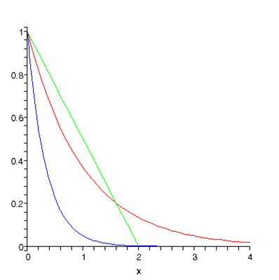
An important definite integral (one with limits) is

$\int_{0}^{\infty} e^{- a x} d x = \frac{1}{a} .$

Notice the minus sign in the exponent: we need an integrand that decreases as $x$ goes towards infinity, otherwise the integral will itself be infinite.

To visualize this result, we plot below $e^{- x}$ and $e^{- 3 x} .$ Note that the green line forms the hypotenuse of a right-angled triangle of area 1, and it is very plausible from the graph that the total area under the $e^{- x}$ curve is the same, that is, 1, as it must be. The $e^{- 3 x}$ curve has area 1/3 under it, ( $a = 3$ ).

Now for something a bit more challenging: how do we evaluate the integral

$I (a) = \int_{- \infty}^{\infty} e^{- a x^{2}} d x ?$

( $a$ has to be positive, of course.) The integral will definitely not be infinite: it falls off equally fast in both positive and negative directions, and in the positive direction for $x$ greater than 1, it’s smaller than $e^{- a x},$ which we know converges.

To see better what this function looks like, we plot it below for $a = 1$ and $a = 4$ :

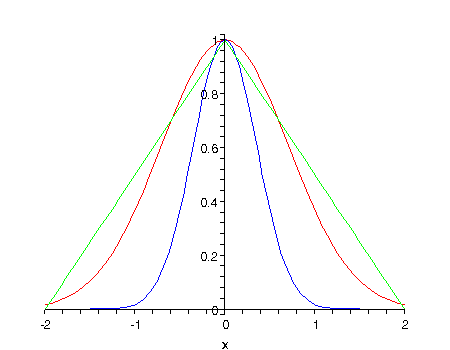
Notice first how much faster than the ordinary exponential $e^{- x}$ this function falls away. Then note that the blue curve, $a = 4,$ has about half the total area of the $a = 1$ curve. In fact, the area goes as $1 / \sqrt{a} .$ The green lines help see that the area under the red curve (positive plus negative) is somewhat less than 2, in fact it’s $\sqrt{π} = 1.77$ approximately.

But $—$ it’s not so easy to evaluate! There is a trick: square it. That is to say, write

${(I (a))}^{2} = \int_{- \infty}^{\infty} e^{- a x^{2}} d x \int_{- \infty}^{\infty} e^{- a y^{2}} d y .$

Now, this product of two integrals along lines, the $x$ -integral and the $y$ -integral, is exactly the same as an integral over a plane, the $(x, y)$ plane, stretching to infinity in all directions. We can rewrite it

$\int_{- \infty}^{\infty} e^{- a x^{2}} d x \int_{- \infty}^{\infty} e^{- a y^{2}} d y = \int_{- \infty}^{\infty} \int_{- \infty}^{\infty} e^{- a x^{2}} e^{- a y^{2}} d x d y = \int_{- \infty}^{\infty} \int_{- \infty}^{\infty} e^{- a r^{2}} d x d y$ ,

$r$ is just the distance from the origin $(0, 0)$ in the $(x, y)$ plane. The plane is divided up into tiny squares of area $d x d y,$ and doing the integral amounts to finding the value of $e^{- a r^{2}}$ for each tiny square, multiplying by the area of that square, and adding the contributions from every square in the plane.

At first glance, this approach is no easier than the original problem—but then we see that the integrand $e^{- a r^{2}}$ has a circular symmetry: for any circle centered at the origin (0, 0), it has the same value anywhere on the circle. To exploit this, we shouldn’t be dividing the (x, y) plane up into little squares at all, we should be dividing it into regions, each having all points close to the same distance from the origin.

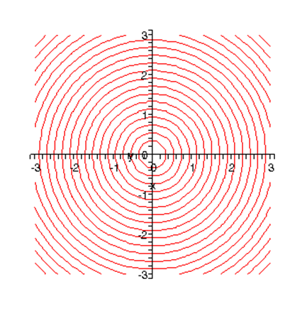
These are called “annular” regions: the area between two circles, both centered at the origin, the inner one of radius $r,$ the slightly bigger outer one having radius $r + d r .$ We take $d r$ to be very small, so this is a thin circular strip, of length $2 π r$ (the circumference of the circle) and breadth $d r,$ and therefore its total area is $2 π r d r$ (neglecting terms like $d r^{2},$ which become negligible for $d r$ small enough).

So, the contribution from one of these annular regions is $e^{- a r^{2}} 2 π r d r,$ and the complete integral over the whole plane is:

${(I (a))}^{2} = π \int_{0}^{\infty} e^{- a r^{2}} 2 r d r .$

This integral is easy to evaluate: make the change of variable to $u = r^{2}, d u = 2 r d r,$ giving

${(I (a))}^{2} = π \int_{0}^{\infty} e^{- a u} d u = \frac{π}{a},$

so taking square roots

$I (a) = \int_{- \infty}^{\infty} e^{- a x^{2}} d x = \sqrt{\frac{π}{a}} .$

Some Integrals Useful in the Kinetic Theory of Gases

We can easily generate more results by differentiating $I (a)$ above with respect to the constant $a$ !

Differentiating once:

$\frac{d}{d a} \int_{- \infty}^{\infty} e^{- a x^{2}} d x = - \int_{- \infty}^{\infty} x^{2} e^{- a x^{2}} d x = \frac{d}{d a} \sqrt{\frac{π}{a}} = - \frac{1}{2 a} \sqrt{\frac{π}{a}}$

and differentiating this result with respect to $a$ gives

$\int_{- \infty}^{\infty} x^{4} e^{- a x^{2}} d x = \frac{3}{4 a^{2}} \sqrt{\frac{π}{a}} .$

The ratio of these two integrals comes up in the kinetic theory of gases in finding the average kinetic energy of a molecule with Maxwell’s velocity distribution.

$\frac{\int_{- \infty}^{\infty} x^{4} e^{- a x^{2}} d x}{\int_{- \infty}^{\infty} x^{2} e^{- a x^{2}} d x} = \frac{\frac{3}{4 a^{2}} \sqrt{\frac{π}{a}}}{\frac{1}{2 a} \sqrt{\frac{π}{a}}} = \frac{3}{2 a} .$

Finding this ratio without doing the integrals: It is interesting to note that this ratio could have been found with much less work, in fact without evaluating the integrals fully, as follows: Make the change of variable $y^{2} = a x^{2}$ , so $d y = \sqrt{a} d x$

and

$\int_{- \infty}^{\infty} x^{2} e^{- a x^{2}} d x = {(a)}^{- 3 / 2} \int_{- \infty}^{\infty} y^{2} e^{- y^{2}} d y = C a^{- 3 / 2}$

where $C$ is a constant independent of $a,$ because $a$ has completely disappeared in the integral over $y .$ (Of course, we know $C = \sqrt{π} / 2,$ but that took a lot of work.) Now, the integral with $x^{4}$ for the leading term in place of $x^{2}$ is given by differentiating the $x^{2}$ integral with respect to $a,$ and multiplying by $- 1,$ as discussed above, so, differentiating the right hand side of the above equation, the $x^{4}$ integral is just $(3 / 2) C a^{- 5 / 2},$ and the $C$ cancels out in the ratio of the integrals.

However, we do need to do the integrals at one point in the kinetic theory: the overall normalization of the velocity distribution function is given by requiring that

$1 = \int_{0}^{\infty} f (v) d v = \int_{0}^{\infty} 4 π A^{3} v^{2} e^{- m v^{2} / 2 k T}$

using the results we found above, giving

$f (v) = 4 π {(\frac{m}{2 π k T})}^{3 / 2} v^{2} e^{- m v^{2} / 2 k T} .$

One last trick…

We didn’t need this in the kinetic theory lecture, but is seems a pity to review exponential integrals without mentioning it.

It’s easy to do the integral

$I (a, b) = \int_{- \infty}^{\infty} e^{- a x^{2}} e^{b x} d x .$

It can be written

$I (a, b) = \int_{- \infty}^{\infty} e^{- a {(x - b / 2 a)}^{2}} e^{b^{2} / 4 a} d x = e^{b^{2} / 4 a} \int_{- \infty}^{\infty} e^{- a {(x - b / 2 a)}^{2}} d x = e^{b^{2} / 4 a} \sqrt{π / a}$

where to do the last step just change variables from $x$ to $y = x - b / 2 a .$

This can even be used to evaluate for example

$\int_{- \infty}^{\infty} e^{- a x^{2}} \cos b x d x$

by writing the cosine as a sum of exponentials.

previous index next