Molecular Collisions

Michael Fowler

Difficulties Getting the Kinetic Theory Moving

Oddly, the first published calculation of the average speed of a molecule in the kinetic theory of gases appeared in the Railway Magazine, of all places, in 1836. Why there? Well, the calculation was by John Herapath $—$ he owned the magazine. He was definitely not part of the scientific establishment: a previous paper of his on the kinetic theory had been rejected by the Royal Society. But the calculation of molecular speed was in fact correct. Another outsider, John James Waterston, submitted an excellent paper on the kinetic theory to the Royal Society in 1846, to have it rejected as “nonsense”. This was evidently still the age of the caloric theory, at least in the Royal Society. In 1848, Joule (who had worked with Herapath, and was also something of an outsider) presented a paper at a meeting of British Association where he announced that of the speed of hydrogen molecules at 60˚F was about 1 mile per second, close to correct. Again, though, this did not excite wide interest…

Finally, in 1857, a pillar of the scientific establishment $—$ Clausius $—$ wrote a paper on the kinetic theory, repeating once more the calculation of average molecular speed (around 460 meters per second for room temperature oxygen molecules). He mentioned the earlier work by Joule, and some more recent similar calculations by Krönig. Suddenly people sat up and took notice! If a highly respected German professor was willing to entertain the possibility that the air molecules in front of our faces were mostly traveling faster than the speed of sound, perhaps there was something to it…

How Fast Are Smelly Molecules?

But there were obvious objections to this vision of fast molecules zipping by. As a Dutch meteorologist, C. H. D. Buys-Ballot, wrote: [if the molecules are traveling so fast] how does it then happen that tobacco-smoke, in rooms, remains so long extended in immoveable layers?” (Nostalgia trip for smokers!) He also wondered why, if someone opens a bottle of something really smelly, like ammonia, you don’t smell it across the room in a split second, if the molecules are moving so fast. And, why do gases take ages to intermingle?

These were very good questions, and forced Clausius to think about the theory a bit more deeply. Buys-Ballot had a point: at that speed, the smelly NH₃’s really would fill a whole room in moments. So what was stopping them? The speed of the molecules follows directly from measuring the pressure and density $—$ you don’t need to know the size of molecules. If the kinetic theory is right at all, this speed has to be correct. Assuming, then, the speed is more or less correct, the molecules are evidently not going in straight lines for long. They must be bouncing off the other molecules. Still, the standard kinetic theory pressure calculation assumed each molecule to be bouncing from wall to wall inside the box, collisions with the other molecules had always been ignored, because the molecules were so tiny. Evidently, though, they weren’t.

The Mean Free Path

Clausius concluded that the molecules must be big enough to get in each other’s way to some extent. He assumed the average speed calculation was still about right, and that the molecules only interacted when they were really close. So, watching one molecule, most of the time it’s going in a straight line, not influenced by the other molecules, then it gets close to another one and bounces off in a different direction. He termed the average distance between collisions the mean free path.

But how could this be reconciled with the pressure calculation, the pressure from a single molecule being found by counting the times per second it bounced off a given wall? Evidently each molecule will now take a lot longer to get across the container $—$ will that lower the pressure? The answer is no: although molecules now take a long time to do the round trip, they don’t have to $—$ a molecule bouncing off the wall can hit another nearby molecule and go straight back to the wall. The pressure on a wall depends on the density of molecules close to the wall (less than of order a mean free path away), and their velocity distribution. This won’t be too different from the no-collisions case.

Gas Viscosity Doesn’t Depend on Density!

This fixed up the theory in the sense of answering Buys-Ballot’s objections, but it turned out to do much more. Maxwell took the concept of mean free path, and used it to prove the viscosity of a gas should be independent of density over a very wide range. (Viscosity arises when fast molecules move into a slower stream: halving the density halves the number of fast molecules getting over, but they get twice as far, so penetrate into even slower streams. For a much more detailed explanation, see my lecture on viscosity.) Maxwell was startled (his word: Phil. Mag, Jan-Jun 1860, p 391) by this result, and thought it probably spelled doom for the kinetic theory, because it contradicted experimental findings. But the experiments, it turned out, were not very good, and had found the (wrong) answer they expected. Maxwell did the experiments more carefully himself, and found agreement with the kinetic theory $—$ the viscosity really didn’t depend on density! Usually in physics good experiments knock down bad theories $—$ this time it was the other way round.

Gas Diffusion: the Pinball Scenario: Finding the Mean Free Path in Terms of the Molecular Diameter

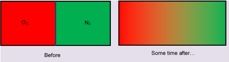
How does the mean free path picture handle mutual diffusion of two gases, say oxygen and nitrogen, when a partition initially separating them is removed?

To see a molecular animation, click here!

For a box holding a few liters, it takes of the order an hour or so for the gases to mix. (We’re assuming the temperature is kept constant so that convection currents don’t arise $—$ such currents would reduce the time substantially.) Obviously, the rate of mixing must depend on the mean free path: if it was centimeters, the mixing would be pretty complete in milliseconds. In fact, as we shall see, the mean free path can be deduced from the measured rate of penetration of one gas by the other.

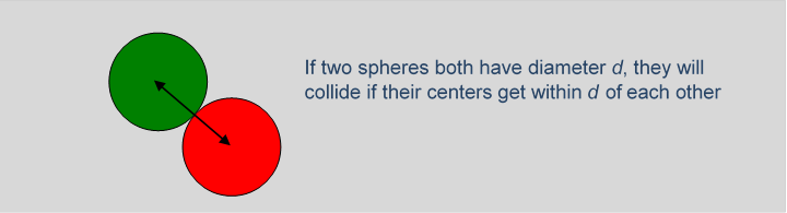
First, though, we’ll show how to derive the mean free path in units of the diameter of the molecules, taking O₂ and N₂ to be spheres of diameter $d .$ (You’re used to seeing them pictured like dumbbells and that’s true of the two nuclei, but the surrounding electron cloud is in fact close to spherical.)

Think of one of the oxygen molecules moving into nitrogen. So now visualize the little O₂ sphere shooting into this space where all these other spheres are moving around. Temporarily, for ease of visualization, let’s imagine all the other spheres to be at rest. This is a pinball machine scenario:

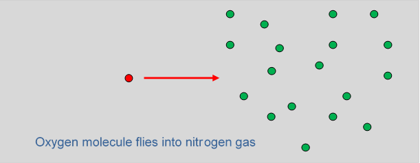
How far can we expect the O₂ to get before it hits an N₂? The average distance into the gas before a collision is the mean free path. Let’s try to picture how much room there is to fly between these fixed N₂ spheres. (Bear in mind that the picture above should be three-dimensional!) We do know that if it were liquid nitrogen, there would be very little room: liquids are just about incompressible, so the molecules must be touching. Roughly speaking, a molecule of diameter $d$ will occupy a cubical volume of about $d^{3}$ (there has to be some space left over $—$ we can pack cubes to fill space, but not spheres.)

We also know that liquid nitrogen weighs about 800 kg per cubic meter, whereas N₂ gas at room temperature (and pressure) weighs about 1.2 kg per cubic meter, a ratio of 670. This means that on average each molecule in the gas has 670 times more room $—$ that is, it has a space 670 times the volume $d^{3}$ we gave it in the liquid. So in the gas, the average center-to-center separation of the molecules will be the cube root of 670, which is about $8.75 d .$ So the picture is a gas of spheres of diameter $d,$ placed at random, but separated on average by distances of order $10 d .$ It’s clear that shooting an oxygen molecule into this it will get quite a way. Let us emphasize again that this picture is independent of the actual size of $d :$ we’re only considering the ratio of mean free path to molecular diameter.

We now estimate just how far an O₂ will get, on average, as it shoots into this forest of spheres. Picture the motion of the center of the oxygen molecule. Before any collision, it will be moving on a straight-line path. Just how close does the O₂ center have to get to an N₂ center for a hit? Taking both O₂, N₂ to be spheres of diameter $d,$ if an N₂ center lies within $d$ of the O₂ center’s path, there will be a hit.

Note: this picture is simplified in that we’re taking the molecules to be hard spheres. This is not a bad approximation, but the repulsive potential does not fall quite that suddenly, and consequently the effective scattering size varies somewhat with speed, i.e. with temperature. This turns out to be important in finding the temperature dependence of viscosity, for example.

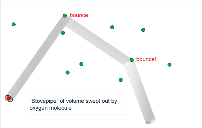
So we can think of the O₂ as sweeping out a volume, a cylinder of radius $d$ centered on its path, hitting and deflecting if it encounters an N₂ centered within that cylinder. So how far will it get, on average, before a hit? In traveling a distance $x,$ it sweeps out a volume $π d^{2} x .$ Now picture it going through the gas for some considerable length of time, so there are many collisions. The volume swept out will look like a stovepipe, long straight cylindrical sections connected by elbows at the collisions. The total volume of this stovepipe (ignoring tiny corrections from the elbows) will be just $π d^{2} L,$ $L$ being the total length, that is, the total distance the molecule traveled.

If the density of the nitrogen is $n$ molecules per cubic meter, the number of N₂’s in this stovepipe volume will be $π d^{2} L n,$ in other words, this will be the number of collisions. Therefore, the average distance between collisions, the mean free path $l,$ is given by:

$mean free path l = \frac{total distance traveled}{number of collisions} = \frac{L}{π d^{2} L n} = \frac{1}{π d^{2} n} .$

So what is $n$ ? We estimated above that each molecule has space $670 d^{3}$ to itself, so $n$ is just how many of those volumes there are in one cubic meter, that is, $n = 1 / 670 d^{3} .$

Therefore, the mean free path is given by

$l = \frac{1}{π d^{2} n} = \frac{670 d^{3}}{π d^{2}} \approx 200 d .$

(We can see from this that the average length of stovepipe sections between elbows is 200 times the pipe radius, so neglecting any volume corrections from the elbows was an excellent approximation, and our diagram has the sections far too short compared with the diameter.)

Notice that this derivation of the mean free path in terms of the molecular diameter depends only on knowing the ratio of the gas density to the liquid density $—$ it does not depend on the actual size of the molecules!

But it does mean that if we can somehow measure the mean free path, by measuring how fast one gas diffuses into another, for example, we can deduce the size of the molecules, and historically this was one of the first ways the size of molecules was determined, and so Avogadro’s number was found.

But the Pinball Picture is Too Simple: the Target Molecules Are Moving!

There is one further correction we should make. We took the N₂ molecules to be at rest, whereas in fact they’re moving as fast as the oxygen molecule, approximately. This means that even if the O₂ is temporarily at rest, it can undergo a collision as an N₂ comes towards it. Clearly, what really counts in the collision rate is the relative velocity of the molecules.

Defining the average velocity as the root mean square velocity, if the O₂ has velocity ${\vec{v}}_{1}$ and the N₂ ${\vec{v}}_{2}$ , then the square of the relative velocity

$\bar{{({\vec{v}}_{1} - {\vec{v}}_{2})}^{2}} = \bar{{\vec{v}}_{1}^{2}} - 2 \bar{{\vec{v}}_{1} \cdot {\vec{v}}_{2}} + \bar{{\vec{v}}_{2}^{2}} = \bar{{\vec{v}}_{1}^{2}} + \bar{{\vec{v}}_{2}^{2}},$

since $\bar{{\vec{v}}_{1} \cdot {\vec{v}}_{2}}$ must average to zero, the relative directions being random. So the average square of the relative velocity is twice the average square of the velocity, and therefore the average root-mean-square velocity is up by a factor $\sqrt{2},$ and the collision rate is increased by this factor. Consequently, the mean free path is decreased by a factor of $\sqrt{2}$ when we take into account that all the molecules are moving.

Our final result, then, is that the mean free path

$l = \frac{1}{\sqrt{2} π d^{2} n} .$

Finding the mean free path is $—$ literally $—$ the first step in figuring out how rapidly the oxygen atoms will diffuse into the nitrogen gas, and of course vice versa.

If Gases Intermingle 0.5cm in One Second, How Far in One Hour?

What we really want to know is just how much we can expect the gases to have intermingled after a given period of time. We’ll just follow the one molecule, and estimate how far it gets. To begin with, let’s assume for simplicity that it tales steps all of the same length $l,$ but after each collision it bounces off in a random direction. So after $N$ steps, it will have moved to a point

$\vec{L} = {\vec{l}}_{1} + {\vec{l}}_{2} + {\vec{l}}_{3} + \dots + {\vec{l}}_{N},$ ,

where each vector ${\vec{l}}_{j}$ has length $l,$ but the vectors all point in random different directions.

If we now imagine many of the oxygen molecules following random paths like this, how far on average can we expect them to have drifted after $N$ steps? (Note that they could with equal likelihood be going backwards!) The appropriate measure is the root-mean-square distance,

$\bar{{\vec{L}}^{2}} = \bar{{({\vec{l}}_{1} + {\vec{l}}_{2} + {\vec{l}}_{3} + \dots {\vec{l}}_{N})}^{2}} = N l^{2} + \sum_{i, j} \bar{{\vec{l}}_{i} \cdot {\vec{l}}_{j}} .$

Since the direction after each collision is completely random, $\bar{{\vec{l}}_{i} \cdot {\vec{l}}_{j}} = 0,$ and the root-mean-square distance

$\sqrt{\bar{{\vec{L}}^{2}}} = \sqrt{N} l .$ .

If we allow steps of different lengths, the same argument works, but now $l$ is the root-mean-square path length. The important factor here is the $\sqrt{N} .$

This means that the average distance diffused in one second is $\sqrt{10^{10}} l = 10^{5} l,$ say half a centimeter (justified in the next section). The average distance in one hour would be only 60 times this, or 30 cm., and in a day about a meter and a half $—$ the average distance traveled is only increasing as the square root of the time elapsed!

This is a very general result. For example, suppose we have a gas in which the mean free path is $l$ and the average speed of the molecules is $v .$ Then the average time between collisions $τ = l / v .$ The number of collisions in time $t$ will be $t / τ,$ so the average distance a molecule moves in time $t$ will be $r = l \sqrt{t / τ} .$

Actually Measuring Mean Free Paths

It should be clear from the above that by carefully observing how quickly one gas diffuses into another, the mean free path could be estimated. Obviously, oxygen and nitrogen are not the best candidates: to see what’s going on, a highly visible gas like bromine diffusing into air would be more practical. However, there’s a better way to find the mean free path. As we proved in the lecture on viscosity, the viscosity coefficient $η = \frac{1}{3} n m v l,$ where $n$ is the number density, $m$ the molecular mass, $v$ the average speed and $l$ the mean free path. The viscosity can be measured quite accurately, the mean free path in air was found to be $l \approx 60 nm ,$ or $6 \times 10^{- 8} m .$

In 1865, Josef Loschmidt gave the first good estimate of the size of molecules. He used the viscosity data to find the mean free path, assumed as we did above that the molecules were more or less touching each other in the liquid, then used the geometric argument above to nail down the ratio of molecular size to mean free path. He overestimated by a factor of three or so, but this was much closer to the truth than anyone else at the time.

Here are some numbers: for O₂, N₂, $d \approx 0.3 nm ,$ $l \approx 60 nm,$ the speed of the molecules at room temperature $v$ is approximately 500 meters per sec., so the molecule has of order 10¹⁰ collisions per second.

Why did Newton get the Speed of Sound Wrong?

A famous mystery cleared up by arguments like this was that Newton predicted the speed of sound would be given by $c^{2} = B / ρ,$ as we discussed earlier in the course, with $B$ the bulk modulus. But when $B$ was measured carefully by slowly compressing air, the result was in error by about 30%! The speed of sound predicted a higher (stiffer) bulk modulus.

The explanation turned out to be that in a slow measurement of the bulk modulus, the gas stays at the same temperature $—$ the heating caused by slow compression leaks away. But if the compression is rapid, the gas heats up and so the pressure goes up more than if it had stayed at the same temperature. So the question is whether the compression and decompression as a sound wave passes through is so rapid that the heated-up gas doesn’t have time to spread to the cooled regions. For sound at say 1000Hz, the wavelength is 34 cm. If compression heats gas locally, the hot molecules will diffuse away in a similar manner to that discussed above. They will be slightly faster than the average molecules. In 1/1000 th of a second, they will have 10⁷ collisions, so will travel about $\sqrt{10^{7}} l \approx 3000 l \approx 0.2 mm .$ This tiny distance compared with the wavelength of the sound wave means that during the compression/decompression cycles as the wave passes through, the heat has no chance to dissipate $—$ so, effectively, it’s like compressing a gas in an insulated container, it’s harder to compress than it would be if the heat generated could flow away, and the bulk modulus is higher by an amount (around 30%) we shall work out in a forthcoming lecture.

previous index next