Calculating Viscous Flow: Velocity Profiles in Rivers and Pipes

Michael Fowler

Introduction

In this lecture, we’ll derive the velocity distribution for two examples of laminar flow. First we’ll consider a wide river, by which we mean wide compared with its depth (which we take to be uniform) and we ignore the more complicated flow pattern near the banks. Our second example is smooth flow down a circular pipe. For the wide river, the water flow can be thought of as being in horizontal “sheets”, so all the water at the same depth is moving at the same velocity. As mentioned in the last lecture, the flow can be pictured as like a pile of printer paper left on a sloping desk: it all slides down, assume the bottom sheet stays stuck to the desk, each other sheet moves downhill a little faster than the sheet immediately beneath it. For flow down a circular pipe, the laminar “sheets” are hollow tubes centered on the line down the middle of the pipe. The fastest flowing fluid is right at that central line. For both river and tube flow, the drag force between adjacent small elements of neighboring sheets is given by force per unit area

$\frac{F}{A} = η \frac{d v (z)}{d z}$

where now the $z$ -direction means perpendicular to the small element of sheet.

A Flowing River: Finding the Velocity Profile

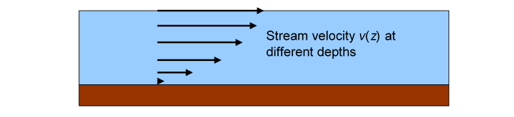
For a river flowing steadily down a gentle incline under gravity, we’ll assume all the streamlines point in the same direction, the river is wide and of uniform depth, and the depth is much smaller than the width. This means almost all the flow is well away from the edges (the river banks), so we’ll ignore the slowing down there, and just analyze the flow rate per meter of river width, taking it to be uniform across the river.

The simplest basic question is: given the slope of the land and the depth of the river, what is the total flow rate?

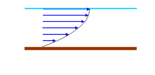
To answer, we need to find the speed of flow $v (z)$ as a function of depth (we know the water in contact with the river bed isn’t flowing at all), and then add the flow contributions from the different depths (this will be an integral) to find the total flow. The function $v (z)$ is called the “velocity profile”. We’ll prove it looks something like this:

(For a smoothly flowing river, the downhill ground slope would be imperceptible on this scale.)

But how do we begin to calculate $v (z)$ ?

Recall that (in an earlier lecture) to find how hydrostatic pressure varied with depth, we mentally separated a cylinder of fluid from its surroundings, and applied Newton’s Laws: it wasn’t moving, so we figured its weight had to be balanced by the sum of the pressure forces it experienced from the rest of the fluid surrounding it. In fact, its weight was balanced by the difference between the pressure underneath and that on top.

Taking a cue from that, here we isolate mentally a thin layer of the river, like one of those sheets of printer paper, lying between height $z$ above the bed and $z + Δ z .$ This layer is moving, but at a steady speed, so the total force on it will still be zero. Like the whole river, this layer isn’t quite horizontal, its weight has a small but nonzero component dragging it downhill, and this weight component is balanced by the difference between the viscous force from the faster water above and that from slower water below.

Bear in mind that the diagram below is at a tiny angle $θ$ to the horizontal:

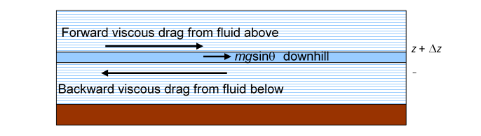
Obviously, for the forces to balance, the backward drag on the thin layer from the slower moving water beneath has to be stronger than the forward drag from the faster water above, so the rate of change of speed with height above the river bed is decreasing on going up from the bed.

Let us find the total force (which must be zero) on one square meter of the thin layer of water between heights $z$ and $z + Δ z :$

First, gravity: if the river is flowing downhill at some small angle $θ,$ this square meter of the layer (volume $Δ z m \times 1 m^{2} = Δ z m^{3}$ , density $ρ$ ) experiences a gravitational force $m g \sin θ \approx ρ g Δ z \cdot θ$ tugging it downstream (taking the small angle approximation, $\sin θ = θ$ .)

Next, the viscous drag forces: the square meter of layer experiences two viscous forces, one from the slower water below, equal to $η d v (z) / d z,$ tending to slow it down, one from the faster water above it, $η d v (z + Δ z) / d z,$ tending to speed it up.

Gravity must balance out the difference between the two viscous forces:

$ρ g θ Δ z + η \frac{d}{d z} v (z + Δ z) - η \frac{d}{d z} v (z) = 0$

We can already see from this equation that, unlike the fluid between the plates, $v (z)$ can’t possibly be linear in $z$ $—$ the equation would not balance if $d v / d z$ were the same at $z$ and $z + Δ z$ !

Dividing throughout by $η$ and by $Δ z,$

$ \frac{\frac{d}{d z} v (z + Δ z) - \frac{d}{d z} v (z)}{Δ z} = - \frac{ρ g θ}{η} .$

Taking now the limit $Δ z \to 0,$ and recalling the definition of the differential

$\frac{d f (x)}{d x} = \lim_{Δ x \to 0} \frac{f (x + Δ x) - f (x)}{Δ x}$

we find the differential equation

$\frac{d^{2} v (z)}{d z^{2}} = - \frac{ρ g θ}{η} .$

The solution of this equation is easy:

$v (z) = - \frac{ρ g θ}{2 η} z^{2} + C z + D$

with $C, D$ constants of integration.

Remember that the velocity $v (z)$ is zero at the bottom of the river, $z = 0,$ so the constant must be zero, and can be dropped immediately. But we’re not through $—$ we haven’t found $C .$ To do that, we need to go to the top.

Velocity Profile Near the River Surface

What happens to the thin layer of river water at the very top $—$ the layer in contact with the air? Assuming there is negligible wind, there is essentially zero parallel-to-the-surface force from above.

So the balance of forces equation for the top layer is just

$ρ g θ Δ z - η \frac{d}{d z} v (z) = 0 .$

We can take this top layer to be as thin as we like, so let’s look what happens in the limit of extreme thinness, $Δ z \to 0.$ . The term $ρ g θ Δ z$ then goes to zero, so the other term must as well. Since $η$ is constant, this means

$\frac{d}{d z} v (z) = 0 at the surface z = h .$

So the velocity profile function $v (z)$ has zero slope at the river surface.

With this new information, we can finally fix the arbitrary integration constant $C .$

Now the velocity profile

$v (z) = - \frac{ρ g θ}{2 η} z^{2} + C z,$

$\frac{d v (z)}{d z} = - \frac{ρ g θ}{η} z + C,$

and $\frac{d}{d z} v (z = h) = 0$ gives $C = \frac{ρ g θ h}{η} .$

Putting this value for $C$ into $v (z)$ we have the final result:

$v (z) = \frac{ρ g θ}{2 η} z (2 h - z) .$

This velocity profile $v (z)$ is half the top part of a parabola:

Total River Flow

Knowing the velocity profile $v (z)$ enables us to compute the total flow of water in the river. As explained earlier, we’re assuming a wide river having uniform depth, ignoring the slowdown near the edges of the river, taking the same $v (z)$ all the way across. We’ll calculate the flow across one meter of width of the river, so the total flow is our result multiplied by the river’s width.

The flow contribution from a single layer of thickness $Δ z$ at height $z$ is $v (z) Δ z$ cubic meters per second across one meter of width. The total flow is the sum over all layers. In the limit of many infinitely thin layers, that is, $Δ z \to 0,$ the sum becomes an integral, and the total flow rate

$I = \int_{0}^{h} v (z) d z = \int_{0}^{h} (ρ g θ / 2 η) z (2 h - z) d z = (ρ g θ / 3 η) h^{3}$

where $h$ is the depth of the river. So, if there’s a storm and the river is twice as deep as normal, and flowing steadily, the flow rate will be eight times normal.

Exercise: plot on a graph the velocity profiles for two rivers, one of depth $h$ and one $2 h,$ having the same values of $ρ, g, θ and η .$ What is the ratio of the surface velocities of the two rivers? Suppose that one meter below the surface of one of the rivers, the water is flowing 0.5 m.sec^-1 slower than it is flowing at the surface. Would that also be true of the other river?

Flow down a Circular Tube (Poiseuille Flow)

The flow rate for smooth flow through a pipe of circular cross-section can be found by essentially the same method. (This was the flow pattern analyzed by Poiseuille and used by him to confirm Newton’s postulate of fluid flow behavior being governed by a coefficient of viscosity.)

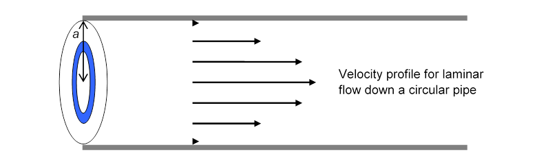
In the pipe, the flow is fastest in the middle, and the water in contact with the pipe wall (like that at the river bed) doesn’t flow at all. The river’s flow pattern was most naturally analyzed by thinking of flat layers of water, all the water in one layer having the same speed. What would be the corresponding picture for flow down a pipe? Here all the fluid at the same distance from the center moves down the pipe at the same speed $—$ instead of flat layers of fluid, we have concentric hollow cylinders of fluid, one inside the next, with a tiny rod of the fastest fluid right at the center. This is again laminar flow, even though this time the “sheets” are rolled into tubes. The blue circular area on the cross-section of the pipe shown below represents one of these cylinders of fluid $—$ all the fluid between $r$ and $r + Δ r$ from the central line.

Each of these hollow cylinders of water is pushed along the pipe by the pressure difference between the ends of the pipe. Each feels viscous forces from its two neighboring cylinders: the next bigger one, which surrounds it, tending to slow it down, but the next smaller one (inside it) tending to speed it up. Writing down the differential equation is a little more tricky that for the river, because we must take into account that the two surfaces of the hollow cylinder (inside and outside) have different areas, $2 π r L$ and $2 π (r + Δ r) L .$ It turns out that the velocity profile is again parabolic: the details are given below.

Circular Pipe Flow: Mathematical Details

Suppose the pipe has radius $a,$ length $L$ and pressure drop $Δ P,$

$pressure drop per meter = Δ P / L .$

Let us focus on the fluid in the cylinder between $r$ and $r + Δ r$ from the line down the middle, and we’ll take the cylinder to have unit length, for convenience.

The pressure force maintaining the fluid motion is the difference between pressure x area for the two ends of this one meter long hollow cylinder:

$net pressure force = \frac{Δ P}{L} \cdot 2 π r Δ r .$

(We’re assuming $Δ r ≪ r,$ since we’ll be taking the $Δ r \to 0$ limit, so the end area $≅ 2 π r Δ r .$ The equality becomes exact in the limit.)

This force exactly balances the difference between the outer surface viscous drag force from the slower surrounding fluid and the inner viscous force from the central faster-moving fluid, very similar to the situation in the previous analysis of river flow.

Using $F / A = η d v (z) / d z,$ and remembering that the inner and outer surfaces of the cylinder have slightly different areas, that $Δ P$ is positive, but $d v / d r$ is negative, the force equation is:

$\frac{Δ P}{L} \cdot 2 π r Δ r = - 2 π (r + Δ r) η \frac{d v (r + Δ r)}{d r} + 2 π r η \frac{d v (r)}{d r} .$

Rearranging,

$\begin{matrix} \frac{Δ P}{L} \cdot r = - \frac{(r + Δ r) η \frac{d v (r + Δ r)}{d r} - r η \frac{d v (r)}{d r}}{Δ r} \\ = - η \frac{d}{d r} (r \frac{d v}{d r}) \end{matrix}$

in the limit $Δ r \to 0,$ remembering the definition of the differential (see the similar analysis above for the river).

This can now be integrated to give

$r \frac{d v}{d r} = - \frac{Δ P}{η L} \cdot \frac{r^{2}}{2} + C$

where $C$ is a constant of integration. Dividing both sides by r and integrating again

$v (r) = - \frac{Δ P}{η L} \cdot \frac{r^{2}}{4} + C \ln r + D .$

The constant $C$ must be zero, since physically the fluid velocity is finite at $r = 0.$ The constant $D$ is determined by the requirement that the fluid speed is zero where the fluid is in contact with the tube, at $r = a .$

The fluid velocity is therefore

$v (r) = \frac{Δ P}{η L} \cdot \frac{(a^{2} - r^{2})}{4} .$

To find the total flow rate I down the pipe, we integrate over the flow in each hollow cylinder of water:

$I = \int_{0}^{a} 2 π r v (r) d r = \int_{0}^{a} 2 π \frac{Δ P}{η L} \cdot \frac{(a^{2} r - r^{3})}{4} d r = \frac{π Δ P}{8 η L} \cdot a^{4}$

in cubic meters per second.

Notice the flow rate goes as the fourth power of the radius, so doubling the radius results in a sixteen-fold increase in flow. That is why narrowing of arteries is so serious.

previous index next

Thanks to Linda Fahlberg-Stojanovska for spotting a sign error in the earlier version.