8. The Energy-Time Uncertainty Principle: Decaying States and Resonances

Michael Fowler

Model of a Decaying State

The momentum-position uncertainty principle $Δ p \cdot Δ x \geq ℏ$ has an energy-time analog, $Δ E \cdot Δ t \geq ℏ$ . Evidently, though, this must be a different kind of relationship to the momentum-position one, because $t$ is not a dynamical variable, so this can’t have anything to do with non-commutation.

To illustrate the meaning of the equation $Δ E \cdot Δ t \geq ℏ,$ let us reconsider $α$ -decay, but with a slightly simplified potential to clarify what’s going on. Specifically, we replace the combined nuclear force/electrostatic repulsion barrier with a square barrier, high enough and thick enough that there is a small probability per unit time of the particle tunneling out of the well.

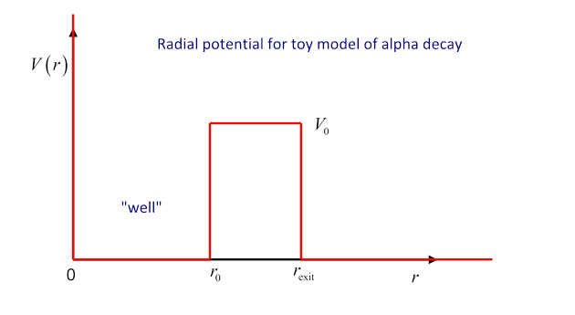
If the barrier thickness were increased to infinity (keeping r₀ fixed) there would be a true bound state having energy $E_{0},$ and for $E_{0}$ well below $V_{0},$ having approximately an integral number of half wavelengths in the well. For a barrier of finite thickness, there is of course some nonzero probability of the particle escaping -- so no longer a true bound state, but for a thick barrier the difference may be hard to detect.

As with the $α$ -decay analysis, we’ll look at this semi-classically, picturing the particle as bouncing off the walls backwards and forwards inside, time $τ$ between hits, and at each hit probability of penetration some small number $ε$ . Therefore, the probability that the particle is still in the well after a time $t = n τ$ is $P (n τ) = {(1 - ε)}^{n}$ . Since $ε$ really is very small for $α$ -decay (less than 10^-12), we can conveniently write $P$ as a function of time by using the formula $e^{- x} = \lim_{ε \to 0} {(1 - ε)}^{x / ε}$ .

From this, the probability of the particle being in the well after $n$ bounces, time $t = n τ,$

$P (t = n τ) = {(1 - ε)}^{n} = {(1 - ε)}^{ε n / ε} ≅ e^{- ε n} .$

The standard notation is to introduce a variable $Γ = ℏ ε / τ$ having the dimensions of energy ( $ε$ being dimensionless), in terms of which

$P (t) ≅ e^{- n ε} = e^{- n Γ τ / ℏ} = e^{- Γ t / ℏ} .$

Evidently $Γ / ℏ$ measures the decay rate. In other words, $Γ / ℏ$ is an inverse lifetime.

The exponential decay law for radioactive elements is completely confirmed experimentally, it is the basis of the “half-life” rule: for any given amount of a radioactive nucleus, half of it will decay in a time period -- the half-life -- fixed for that nucleus.

Obviously, if the modulus of the wave function of the particle in the well is decreasing with time, the time dependence of $ψ$ can no longer be just the $e^{- i E_{0} t / ℏ}$ of the original “bound state”. The wave function inside the well will stay the same shape, but gradually decrease in amplitude:

${| ψ (t) |}^{2} = {| ψ (0) |}^{2} e^{- Γ t / ℏ}$ .

This is a far slower time dependence than that of the $e^{- i E_{0} t / ℏ}$ term, so it is an excellent approximation to put the time dependences together in one exponential factor:

$ψ (t) = ψ (0) e^{- i (E_{0} - i Γ / 2) t / ℏ}$

At this point, the analogy with $Δ p \cdot Δ x \geq ℏ$ emerges. Recall we introduced the $p, x$ uncertainty principle by finding what spread $Δ p$ in the Fourier components of a wave packet were necessary in order for the wave packet to die away from its center over a distance of order $Δ x .$ A true localized wave packet has a continuum of $p$ components, but the right expression for the spread in momentum space $Δ p$ turns out to be given by taking just two waves, $e^{i p x / ℏ}$ and $e^{i (p + Δ p) x / ℏ}$ , and noticing that they fall out of phase in a distance $Δ x \sim ℏ / Δ p$ . The more precise derivation based on Gaussian wave packets reaches essentially the same conclusion.

Now, in the present situation the wave function decays in time rather than space, but the argument is very similar. To construct the decaying wave function we must add together “plane waves in time” $e^{- i E t / ℏ}$ corresponding to different energies. The required spread in energy $Δ E$ follows from an argument just like the one above for space: if the wave function is to be die away in a time of order $Δ t,$ in other words to be “localized in time”, it must be constructed of waves having a range $Δ E$ in energies such that $e^{- i E t / ℏ}$ and $e^{- i (E + Δ E) t / ℏ}$ get out of sync in a time $Δ t .$ This gives immediately $Δ E \cdot Δ t \geq ℏ$ .

It’s worth looking a little further into just what superposition of energy “plane waves” $e^{- i E t / ℏ}$ gives the required exponential-in-time behavior of the wave function for $α$ -decay. Writing

$ψ (t) = ψ (0) \int c (E) e^{- i E t / ℏ} d E / 2 π$

the Fourier coefficients are given by

$c (E) = \int_{0}^{\infty} e^{i (E - E_{0} + i Γ / 2) t / ℏ} d t = \frac{i ℏ}{E - E_{0} + i Γ / 2}$ .

This tells us that the energy with which the $α$ -particle emerges has a probability distribution which is easily normalized to give

${| c (E) |}^{2} = \frac{1}{π} \frac{Γ / 2}{{(E - E_{0})}^{2} + {(Γ / 2)}^{2}} .$

This distribution (called Lorentzian) has a narrow peak of width of order $Γ$ and height of order $1 / Γ$ centered at $E_{0} .$ (Strictly speaking, this is an approximation in that $c (E)$ must of course be zero for $E$ negative -- we ignore that tiny correction here.)

In fact, for the $α$ -decaying nucleus, this energy spread is undetectably small, but that is certainly not the case for other decaying states, where this same analysis applies. In particular, some of the resonant states created in collisions of elementary particles have masses of order 1,000 Mev, and lifetimes of order 10^-23 seconds -- corresponding to a width $Γ$ of the order of 10% of $E_{0}$ ! Obviously, these transient bound states are far from eigenstates of the Hamiltonian $—$ but you will find them listed in particle tables.

Resonances

The time-reversed wave function for $α$ -decay is also a perfectly good solution to Schrödinger’s equation. In principle, if we could arrange for an $α$ -particle to have a spherical ingoing wave function within the narrow energy range corresponding to the quasi bound state, $ψ$ would become very large inside the nucleus, meaning that the $α$ -particle would spend a very long time there compared with the time spent at any other point on the way in: this is called resonance. This particular experiment is never likely to take place, but precisely analogous experiments involving particles scattering off each other, and electrons scattering resonantly from atoms, are common.

One can interpret the wave function for a true bound state as a standing wave, radially containing a whole number of half wavelengths, so that when the wave is reflected at the walls it has just the right phase to interfere constructively with itself. A resonance will have the same wavelength requirement (but the reflection at the walls is of course no longer perfect).

We shall see later that in the case of nonzero angular momentum, the centrifugal barrier provides an effective repulsive term, which together with an attractive force can create a barrier configuration having similar effect to that in the toy model.

It is instructive to use the spreadsheet to discover how the maximum value of ${| ψ |}^{2}$ varies as the barrier height is increased, and to vary the energy to explore how $Γ$ varies with barrier height.

The pictures below are for the energy right at resonance for two different barrier heights. Evidently, if the height of the barrier is increased, ${| ψ |}^{2}$ inside at resonance increases as well. This is easy to understand -- the higher barrier is more difficult to penetrate, so the particle spends even longer inside. The lifetime $Δ t$ is clearly proportional to ${| ψ |}^{2}$ inside.

Important exercise: Open the spreadsheet, find the resonant energy for these cases, and then detune the energy away from resonance. As the energy moves away from resonance, which $ψ$ drops to half its maximum value first?

This energy spread of the resonance is the $Γ$ above, and is related to the “lifetime” of the resonance by $Δ E \cdot Δ t \geq ℏ$ . How does the ratio of the two $Γ$ ’s for these two barriers relate to the ratio of the two maximum values of ${| ψ |}^{2}$ ? Give a physical explanation of your findings.

previous index next PDF