Electrons in One Dimension: the Peierls Transition

Michael Fowler, UVa

Introduction: Looking for Superconductors and Finding Insulators

In 1964, Little suggested (Phys. Rev 134, A1416) that it might be possible to synthesize a room temperature superconductor using organic materials in which the electrons traveled along certain kinds of chains, effectively confined to one dimension.

The first satisfactory theory of “ordinary” superconductivity, that of Bardeen, Cooper and Schrieffer (BCS) had appeared a few years earlier, in 1957. The key point was that electrons became bound together in opposite spin pairs, and at sufficiently low temperatures these bound pairs, being boson like, formed a coherent condensate $—$ all the pairs had the same total momentum, so all traveled together, a supercurrent. The locking of the electrons into this condensate effectively eliminated the usual single-electron scattering by impurities that degrades ordinary currents in conductors.

But what could bind the electrostatically repelling electrons? The answer turned out to be lattice distortions, as first suggested by Fröhlich in 1950. An electron traveling through the crystal attracts the positive ions, the consequent excess of local positive charge attracts another electron. The strength of this binding, and hence the temperature at which the superconducting transition takes place, depends on the rapidity of the lattice response. This was confirmed by the isotope effect: lattice response time obviously depends on the inertia of the lattice, the BCS theory predicted that for a superconducting element with different isotopic varieties, the ratio of the superconducting transition temperatures for pure isotopes $T_{2} / T_{1}$ was equal to $\sqrt{M_{1} / M_{2}}$ , $M_{1}, M_{2}$ being the ion masses, the lighter isotope having the higher transition temperature. This was indeed the case.

Little’s idea was that the build up of positive charge by a passing electron could be speeded up dramatically if instead of having to move ions, it need only rearrange other electrons. Unfortunately, there were no obvious three-dimensional candidate materials. However, if the conduction electrons moved along a one-dimensional chain, polarizable side chains might be attached, and rearrangement of the electronic charge distribution in these side chains would respond very rapidly to a passing conduction electron, building up a local positive charge. If this worked, order of magnitude arguments suggested possible enhancement of the transition temperature by a factor $\sqrt{M / m}$ over ordinary superconductors, $m$ being the electron mass.

In the 1970’s, various organic materials were synthesized and tested, beginning with one called TTF-TCNQ, in which a set of polymer-like long molecules donated electrons to another set, leaving one-dimensional conductors with partially filled bands (see later), seemingly good candidates for superconductivity. Unfortunately, on cooling, these materials surprisingly became insulators rather than superconductors! This was the first example of a Peierls transition, a widespread phenomenon in quasi one-dimensional systems.

The basic mechanism of the Peierls transition can be understood with a simple model. It is a nice example of applied second-order perturbation theory, including the degenerate case. We examine the model and the result below.

It should be added that in some newer materials the Peierls transition is (unexpectedly) suppressed under high pressure, and superconductivity has in fact been observed in organic salts, but so far only at transition temperatures around one Kelvin: Little’s dream is not yet realized.

Second-Order Perturbation Theory: a Periodic Potential in One Dimension

To understand how a one-dimensional conductor might turn into an insulator at low temperatures, we must first become familiar with the simplest model of a one-dimensional conductor:

$H = H^{0} + V = \frac{p^{2}}{2 m} + V (x)$

with $H^{0}$ a gas of noninteracting electrons on a line, and $V$ periodic, that is, $V (x + a) = V (x),$

the potential from a line of ions spaced $a$ apart. We’ll take the system to have $N$ ions in a total length $L,$ so

$L = N a$ and to keep the math simple, we’ll require periodic boundary conditions.

The physics here is that without the potential, the electron eigenstates are plane waves. The effect of the lattice potential is to partially reflect the waves, like a diffraction grating, generating components at different wavelengths. This effect becomes particularly important when the electron wavelength matches twice the ion spacing. For that case, the reflected and original waves have the same strength, the electron is at a standstill. We’ll explore just how this happens later.

The eigenstates of $H^{0}$ are then

${| k 〉}^{(0)} = \frac{1}{\sqrt{L}} e^{i k x}, with e^{i k L} = 1, so k = \frac{2 π n}{L},$

$n$ being an integer. The unperturbed energy eigenvalues,

$H^{0} {| k 〉}^{(0)} = E^{0} {| k 〉}^{(0)}, are just E^{0} = \frac{ℏ^{2} k^{2}}{2 m} .$

(Note: this is to be understood as $H^{0} {| k_{n} 〉}^{(0)} = E_{n}^{0} {| k_{n} 〉}^{(0)}, with E_{n}^{0} = \frac{ℏ^{2} k_{n}^{2}}{2 m} and k_{n} = \frac{2 π n}{L}$ .

We are following standard practice here. We shall also write $\sum_{k} f (k) meaning \sum_{n} f (k_{n})$ . )

It’s worth plotting the (E, k) curve:

Suppose we have ions with two electrons each to contribute to this one-dimensional (supposed) conductor. Assuming they move into these plane wave states, in the system ground state they will fill up the lowest energy states up to a maximum $k -$ value denoted by $\pm k_{F}$ ( $F$ stands for Fermi, this is the Fermi momentum.) Where is it?

We know there will be a total of $2 N$ electrons. We also know that the allowed values of $k,$ from the boundary conditions, are $k_{n} = 2 π n / L$ , with $n$ an integer. In other words, the allowed $k$ ’s are uniformly spaced $2 π / L$ apart, meaning they have a density of $L / 2 π$ in $k -$ space, so the total number between $\pm k_{F}$ is $L k_{F} / π$ . The $2 N$ electrons will have $N$ of each spin, each $k -$ state can take two electrons (one of each spin), so $L k_{F} / π = N = L / a$ , and

$k_{F} = π / a .$

To do perturbation theory, we must find the matrix elements of $V (x)$ between eigenstates of H⁰:

$^{(0)} 〈 k^{'} | V {| k 〉}^{(0)} = \frac{1}{L} \int e^{i (k - k') x} V (x) d x .$

This is just the Fourier component $V_{k - k^{'}}$ of $V (x) .$

If $V (x)$ is periodic with period $a,$

$V_{k} \neq 0 only if k = n K, n an integer, K = 2 π / a .$

In other words, if a function is periodic with spatial period $a,$ the only nonzero Fourier components are those having the same spatial period $a .$

Therefore

$V (x) = \sum_{n} V_{n K} e^{i n K x}, and V_{- n K} = V_{n K}^{*} since V (x) is real; K = 2 π / a .$

The $n = 0$ component of $V (x)$ is of no interest $—$ it is just a constant potential, and so can be taken to be zero. Note that this eliminates the trivial first order correction $E_{k}^{1} =^{(0)} 〈 k | V {| k 〉}^{(0)}$ to the energy eigenvalues.

We shall consider only the components $n = + 1$ and $n = - 1$ of $V (x),$ it turns out that the other components can be treated in similar fashion. For $n = + 1, n = - 1,$ the potential only has nonzero matrix elements between the plane wave state $k$ and $k + K, k - K$ respectively.

So, the second order correction to the energy is:

$\begin{matrix} E_{k}^{2} = \sum_{k^{'} \neq k} \frac{{|^{(0)} 〈 k | V {| k^{'} 〉}^{(0)} |}^{2}}{E_{k}^{0} - E_{k^{'}}^{0}} \\ = \frac{{|^{(0)} 〈 k | V {| k + K 〉}^{(0)} |}^{2}}{E_{k}^{0} - E_{k + K}^{0}} + \frac{{|^{(0)} 〈 k | V {| k - K 〉}^{(0)} |}^{2}}{E_{k}^{0} - E_{k - K}^{0}} \\ = \frac{{| V_{K} |}^{2}}{E_{k}^{0} - E_{k + K}^{0}} + \frac{{| V_{- K} |}^{2}}{E_{k}^{0} - E_{k - K}^{0}} . \end{matrix}$

This result is reasonable provided the terms are small, that is, the energy differences appearing in the denominators are large compared to the relevant Fourier component $V_{K} .$ However, this cannot always be true! Notice that the state $k = π / a$ has exactly the same unperturbed energy $E^{0}$ as the state $k - K = - π / a$ : in this case, nondegenerate perturbation theory is clearly wrong. In fact, even for states close to $k = π / a$ , the energy denominator $E_{k}^{0} - E_{k - K}^{0}$ is small compared with the numerator ${| V_{- K} |}^{2}$ , so the series is not converging.

Quasi-Degenerate Perturbation Theory near the Critical Wavelength

The good news is that, despite the many states near $k = π / a$ and $k = - π / a$ that are close together in energy, for any one state $k$ near $π / a$ the potential only has a nonzero matrix element to one other state close in energy, the state $k - K$ , that is, $k - 2 π / a$ .

The strategy now is to do what might be called quasidegenerate perturbation theory: to diagonalize the full Hamiltonian in the subspace spanned by these two states ${| k 〉}^{(0)}, {| k - K 〉}^{(0)}$ . Other states with nonzero matrix elements to these states are relatively much further away in energy, and can be treated using ordinary perturbation theory.

The matrix elements of the full Hamiltonian in the subspace spanned by these two states are:

$| \begin{matrix} E_{k}^{0} & V_{K}^{*} \\ V_{K} & E_{k - K}^{0} \end{matrix} | .$

Diagonalizing within this subspace gives energy eigenvalues:

$E_{\pm} = \frac{1}{2} (E_{k}^{0} + E_{k - K}^{0}) \pm \sqrt{{(\frac{E_{k}^{0} - E_{k - K}^{0}}{2})}^{2} + | V_{K} |^{2}} .$

Notice that, provided $| E_{k}^{0} - E_{k - K}^{0} | ≫ | V_{K} |$ , to leading order this gives back $E_{\pm} = E_{k}^{0}, E_{k - K}^{0},$ the order depending on $k .$ However, as $k$ approaches $π / a$ , $| E_{k}^{0} - E_{k - K}^{0} |$ becomes of order $| V_{K} |$ , and the energies deviate from the unperturbed values. If $k$ is approaching $π / a$ from below, $E_{k}^{0} < E_{k - K}^{0}$ , and the lower energy is pushed downwards by the perturbation: $E_{k} = E_{-} < E_{k}^{0} .$ This is a common occurrence with almost degenerate states, perturbations cause the energy levels to “repel” each other.

$For k = π / a, E_{k - K}^{0} = E_{k - 2 π / a}^{0} = E_{k}^{0} .$ At this value of $k,$ the unperturbed states are exactly degenerate, and the perturbation lifts the degeneracy to give $E_{\pm} = E_{π / a}^{0} \pm | V_{K} | .$

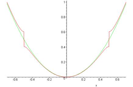
In the graph below, the green (continuous) curve is the unperturbed energy as a function of $k,$ the red curve (with the step) the calculated energy including the leading correction from the periodic potential.

Energy Gaps and Bands

The energy jump, or gap, of $2 | V_{K} |$ at $| k | = π / a$ means that there are no plane wave type eigenstates with energies in that range $—$ attempting to integrate Schrödinger’s equation in the periodic potential for such an energy gives exponentially growing and decaying solutions. Such energy gaps in fact are present in real crystalline solids, the allowed energies are said to be in “bands”. The lowest band for our model is from $k = - π / a to π / a .$ Since the allowed values of $k$ are given by $k = 2 π n / L,$ the spacing between adjacent $k$ ’s is $2 π / L$ and the total number of $k$ ’s in the lowest band is $L / a = N,$ the same as the number of atoms. Since each electron has two spin states, this implies that a one-dimensional crystal of divalent atoms will just fill the lowest band with electrons. Therefore, any outside field can only excite an electron to a different state if an energy of at least $2 | V_{K} |$ is supplied $—$ for a small electric field, the filled band of electrons will remain in the ground state, there will be no current. This material is an insulator.

On the other hand, if monovalent atoms are used, it is clear that the lowest band is only half full, adjacent empty electron states are available. The electrons are free to accelerate if an external field is applied. Barring the unexpected, this one-dimensional crystal would be a metal.

Let us now examine how the periodic potential alters the eigenstates. Ignoring the small corrections from plane waves outside the ${| k 〉}^{(0)}, {| k - K 〉}^{(0)}$ subspace, the eigenstates to this order have the form

$| k 〉 = a_{k} {| k 〉}^{(0)} + a_{k - K} {| k - K 〉}^{(0)}$

where

$\frac{a_{k - K}}{a_{k}} = \frac{E_{-} - E_{k}^{0}}{V_{K}^{*}}$

from the diagonalization of the $2 \times 2$ matrix representing the Hamiltonian in the subspace.

As $k$ increases from 0 towards $π / a,$ the plane wave initially proportional to $e^{i k x}$ has a gradually increasing admixture of $e^{i (k - 2 π / a) x}$ , until at $k = π / a$ the two have equal weight $—$ meaning that the eigenfunction is now a standing wave. In fact, there are two standing wave solutions at $k = π / a$ , corresponding to the energies below and above the gap. Taking the atoms to have an attractive potential, the lower energy wave has a probability distribution peaking at the atomic positions. The diffractive scattering that gives a left-moving component to a right moving wave is known as Bragg scattering. It also manifests itself in the group velocity of the electronic excitations, $v_{group} = d ω / d k = (1 / ℏ) d E / d k .$ An electron injected into a one-dimensional metal would not be a plane wave state, but a wavepacket traveling at the group velocity. It is evident that for an injected electron with mean value of $k$ close to $π / a$ , the electron will move very slowly into the metal. This is to be expected $—$ the eigenstates become standing waves as $k \to π / a .$

For three-dimensional crystals, the situation is far more complicated, but many of the same ideas are relevant. Electron waves are now diffracted by whole planes of atoms, and the three-dimensional momentum space is divided into Brillouin zones, with planes having an energy gap across them.

The Peierls Transition: how Cooling a Conductor Can Give an Insulator

As mentioned in the Introduction, substances very close to monovalent one-dimensional crystals have been synthesized, and it has been found $—$ surprisingly $—$ that at low temperatures many of them undergo a transition from metallic to insulating behavior. What happens is that the atoms in the lattice rearrange slightly, moving from an equally-spaced crystal to one in which the spacing alternates, that is, the atoms form pairs. This is called dimerization, and costs some elastic energy, since for identical atoms the lowest state must be one of equal spacing for any reasonable potential. However, the electrons are able to move to a lower energy state by this maneuver.

Just how this happens can be understood using the perturbation theory analysis above. For equally spaced atoms, the electrons half-fill the band, that is, they fill it up (two electrons, one of each spin, per state) to $| k | = π / 2 a .$

The crucial point is that if the atoms move together slightly into pairs, the crystal has a new period $2 a$ instead of $a .$ This means that the potential now has a nonzero component at $K = - π / a$ , with a nonzero matrix element between the states $k = π / 2 a$ and $k = - π / 2 a$ , and so on. From this point, we can rerun the analysis above, except that now the gaps open up at $| k | = π / 2 a$ instead of at $| k | = π / a .$

The important point is that if the electrons fill all the states to $| k | = π / 2 a$ , and none beyond (as would be the case for monovalent atoms) then the opening of a gap at $| k | = π / 2 a$ means that all the electrons are in states whose energy is lowered. To find the total energy benefit we need to integrate over $k .$

Calculating the Electronic Energy Gained by Doubling the Lattice Period

It is evident from the above that most of the contribution comes from fairly close to $k = π / 2 a$ (and of course symmetrically $k = - π / 2 a$ ). Since we want to find the total lowering in energy, let us study first the bare energy as a function of $k,$ that is, the energy with no potential present. Of course, there isn’t much to say: $E_{k}^{0} = ℏ^{2} k^{2} / 2 m$ . However, the physics of these one-dimensional systems concerns only excitations near the “Fermi surface”, the boundary between filled (low energy) states at zero temperature and empty states. This “Fermi surface” is in fact just two points in one dimension: $k = \pm π / 2 a$ . In the neighborhood of these two Fermi points, it is an excellent approximation to replace the gently curving $E_{k}^{0} = ℏ^{2} k^{2} / 2 m$ by straight line approximations $—$ the slope being $d E / d k = ℏ^{2} k / m = ℏ p / m = ℏ v$ .

Linearizing in the neighborhood of $k = π / 2 a$ , then, we take

$E_{k}^{0} = E_{π / 2 a}^{0} + ℏ v (k - π / 2 a) = E_{π / 2 a}^{0} + ℏ v q$ ,

where

$q = k - π / 2 a,$

just $k$ measured from the Fermi point $π / 2 a$ .

The variable $q$ is negative for the relevant states, since they are on the lower energy side.

The density of states in $k -$ space is a constant $2 \times L / 2 π = L / π$ , remembering the two spin states per $k -$ value.

Recall

$E_{\pm} = \frac{1}{2} (E_{k}^{0} + E_{k - K}^{0}) \pm \sqrt{{(\frac{E_{k}^{0} - E_{k - K}^{0}}{2})}^{2} + | V_{K} |^{2}}$

but now

$K = π / a$

and the lowering of energy of the electrons (counting it as a positive quantity) is:

$2 \int_{0}^{π / 2 a} (E_{k}^{0} - E_{-}) L d k / π = 2 \int (\frac{1}{2} (E_{k}^{0} - E_{k - K}^{0}) + \sqrt{{(\frac{E_{k}^{0} - E_{k - K}^{0}}{2})}^{2} + | V_{K} |^{2}}) L d k / π$

where the extra factor of 2 counts the symmetrical contribution from the left-hand gap. (In examining the above expression, recall that for the $k > 0$ states we are interested in, $k < π / 2 a,$ $E_{k}^{0} - E_{k - K}^{0}$ is negative. The integrand on the right-hand side is still positive, very small for small k, reaching a maximum of $| V_{K} |$ at $k = π / 2 a .$ )

Putting in our linearized energy approximation,

$E_{k}^{0} = E_{π / 2 a}^{0} + ℏ v (k - π / 2 a) = E_{π / 2 a}^{0} + ℏ v q$ ,

and remembering that now $K = π / a,$

$E_{k - K}^{0} = E_{- π / 2 a}^{0} - ℏ v (k + π / 2 a) = E_{- π / 2 a}^{0} - ℏ v q$ .

Since $E_{π / 2 a}^{0} = E_{- π / 2 a}^{0}$ ,

$(E_{k}^{0} - E_{k - K}^{0}) = 2 v ℏ q .$

Substituting these linearized values in the integral for the total energy lowering:

$2 \int_{0}^{π / 2 a} (E_{k}^{0} - E_{-}) L d k / π = 2 \int_{- D}^{0} (v ℏ q + \sqrt{{(v ℏ q)}^{2} + | V_{K} |^{2}}) L d q / π$

where in terms of the variable $q$ we have set the lower limit of integration at $- D$ : we can safely be vague about this lower limit, as the integral turns out to be logarithmic.

Since the integral is over negative numbers, and we have taken the positive square root, it is zero for zero $V_{K},$ as it must be.

The integral can be done exactly, but it is more illuminating to divide the range of integration into $| v ℏ q | \leq | V_{K} |$ and $| v ℏ q | > | V_{K} |$ , then estimate the contributions from these two ranges separately.

First, consider $| v ℏ q | \leq | V_{K} |$ . Here the integrand is of order $| V_{K} |$ , and the region $Δ q$ of integration corresponding to $| v ℏ q | \leq | V_{K} |$ is of order $| V_{K} | / ℏ v,$ so the integral over this range is of order $(L / ℏ v) {| V_{K} |}^{2}$ .

Second, in the region $| v ℏ q | > | V_{K} |$ , we can write

$\begin{array}{l} 2 \int (v ℏ q + \sqrt{{(v ℏ q)}^{2} + | V_{K} |^{2}}) L d q / π = 2 \int (v ℏ q + | v ℏ q | \sqrt{1 + \frac{| V_{K} |^{2}}{{(v ℏ q)}^{2}}}) L d q / π \end{array}$

and expand the square root term. The leading terms cancel since $q$ is negative, and the main contribution comes from the next term. This gives:

$Δ E \approx 2 | V_{K} |^{2} \int_{- D}^{- | V_{K} |} \frac{1}{2 ℏ v} \frac{L d q}{π | q |} = \frac{L | V_{K} |^{2}}{ℏ v} \ln \frac{| V_{K} |}{D} .$

The important thing here is the logarithm. For sufficiently small $| V_{K} |$ , this large (negative) term will dominate any term which is just proportional to $V_{K}^{2}$ . But the elastic energy cost of the lattice “dimerizing” $—$ the atoms forming pairs, so that the distance between atoms alternates on going along the chain $—$ must be proportional to $V_{K}^{2}$ . This leads to the conclusion that some, probably small, dimerization is always going to happen $—$ a one-dimensional equally spaced chain with one electron per ion is unstable.

This dimerization is known as a Peierls transition. Peierls discovered it in the 1930’s when writing a section on one-dimensional models in an introductory solid-state textbook. He put it in the book, but didn’t publish it otherwise. As mentioned in the Introduction, it became very relevant later when some theories suggested that quasi-one-dimensional conductors, materials made up of loosely connected chains, each chain having one electron per atom for a half-filled lowest band, might be high-temperature superconductors. It was found instead that many such materials actually became insulators on cooling: the reason was that at high temperatures, the electrons filled states above and below the point $π / 2 a$ fairly equally, so dimerization did not lower the overall energy much. On lowering the temperature, a point was reached where the Peierls transition gave a lower energy state, and the material became an insulator.

Reference: Rudolf Peierls, More Surprises in Theoretical Physics, Princeton.

previous home next PDF