Boundary Conditions: at the End of the String

Michael Fowler, University of Virginia

Adding Opposite Pulses

Our first move in working with waves was to jiggle the end of a string (or spring) and generate a pulse that we saw traveled along with no perceptible change in shape. We showed that our observation could be expressed mathematically: taking the string initially at rest along the $x$ -axis, its displacement $y$ at point $x$ at time $t$ was evidently described by a function of the form $y = f (x - v t) .$ This function keeps its shape, but as $t$ progresses it moves to the right with speed $v .$

We next analyzed the dynamics of the vibrating string by applying Newton’s Laws of Motion to a little bit of string. This reveals an equation, the wave equation, that any vibration of the string must obey. Reassuringly, our observed form for the moving pulse, $y = f (x - v t),$ does in fact satisfy the wave equation.

The wave equation has one very important property: if you add two solutions to the wave equation, the sum is another solution to the wave equation. This means that if you and a friend send pulses down a rope from the opposite end, the pulses will go right through each other, and when they’re on top of each other, the total displacement of the rope will be just the sum of the displacements corresponding to the individual pulses. We shall see that this gives an important clue for understanding what happens when a pulse reaches the end of the string.

Pulse Reflection

What happens when the pulse gets to the end of the string depends on the end of the string: there are two possibilities:

(a) the end of the string is fixed,

(b) the end of the string is free to move up and down (the pulse corresponds to the string moving in an up-down way).

We refer to these as fixed end and free end boundary conditions.

You may be wondering how the string could have a free end, since it needs to be under tension for the wave to propagate at all. This is arranged by having the string terminate on a ring which is free to move up and down a smooth rod perpendicular to the direction of the string. More important examples of free-end vibrations come up in analyzing musical instruments like the organ, where we shall find that a closed end to an organ pipe is equivalent to a fixed end, an open pipe end is a free end.

An Experiment on Fixed End Reflection and Free End Reflection

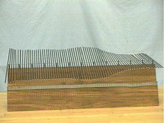
We use a demonstration which has a wire under tension with thin parallel rods perpendicular to the wire attached to it at their centers. The ends of these rods are painted white for visibility, and waves will travel down this array sufficiently slowly to be followed easily. It’s easy to send a pulse down from one end, then either hold the other end fixed or let it move freely, and observe what happens when the pulse reaches the end.

It is found that when the pulse reaches the fixed end, it is reflected with its shape intact, but switched in sign: if before reflection the pulse bulged the string in the $+ y$ direction, after reflection it bulged the string in the $- y$ direction.

However, if the end rod is free to rotate, the pulse is reflected without a change of sign.

Understanding Sign Change in Pulse Reflection

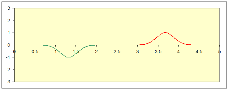
The key to seeing what’s going on when a pulse is reflected is to do a different experiment: send two pulsed down a rope from opposite ends and watch carefully as they pass in the middle. Let’s start with two pulses identical in shape, but of opposite sign. We’ll generate the pulses with a spreadsheet, and watch them as they pass. Remember, the total displacement of the string at any point is the sum of the displacements of the separate pulses.

The two separate pulses look like this:

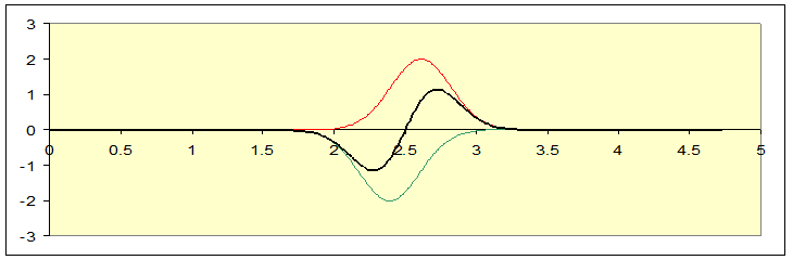
Bearing in mind that the green hides the red along the axis when they’re together, the green and red are separately solutions to the wave equation, the sum of the two pulses is also a solution, and that’s the black line $—$ the actual position of the string at some moment after the pulses are sent on their way $—$ in the diagram below:

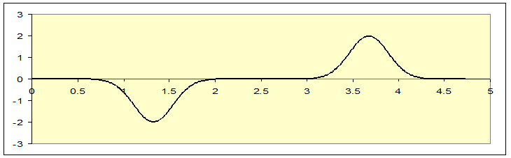
Tracking the two pulses as time goes on, they meet:

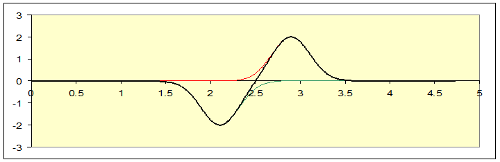
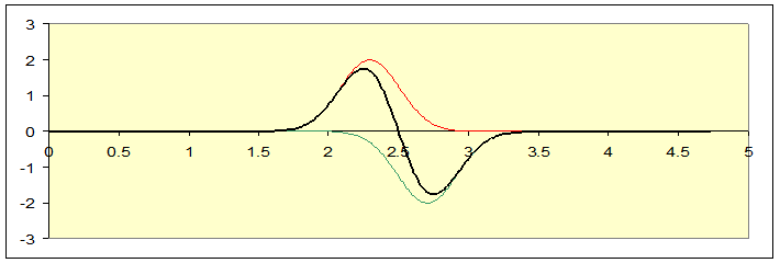
Now we can see the green pulse moving to the right and the red to the left:

They pass (look at the string!):

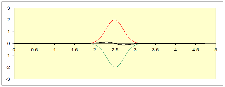
Reviewing this sequence of pictures, notice that the string at the central point, x = 2.5, never moves. It might as well have been nailed in place. Imagine we did nail it in place, chopped off the string to the right of center, and just sent one pulse down from the left-hand end. To see what would happen, we would need to solve the wave equation for the string subject to the fixed end on the right, and a pulse being sent down from the left. But we already know the solution to the wave equation for the whole string with the initial two pulses described above, and the midpoint always stayed fixed. This solution, confined to the left hand half, is to the same equation with the same boundary condition and the same initial configuration as the two pulses on the whole string scenario $—$ so it must be the same solution! We are forced to conclude that when a pulse that curves downwards is sent towards a fixed end, the reflected pulse curves upwards $—$ it just follows the same sequence as the left-hand half in our two pulses full string solution. And, needless to add, this is what we see experimentally.

Free End Boundary Condition

Suppose now in the rod model we send a pulse down from the left, but instead of fixing the rod on the right-hand end, we allow it to rotate freely. What happens? Recall that in deriving the wave equation by writing $F = m a$ for a small piece of string, the accelerating force on the string depended on the small difference in slope of the string at the two ends of the little piece under consideration. Our rod model is a discretized version: for a rod somewhere in the middle, the net force on it depends on the slight difference in slope of the lines connecting it to its neighbors. But for the last rod, if it’s free to move, there’s only a force on one side. For it to have the same acceleration as its neighbors, the force it feels from its only neighbor must be tiny, it must be comparable to the difference in force from typical neighbor rods. This means that the curve made by the dots on the ends of the rods (see photo of equipment) must be essentially horizontal at the end $—$ the last two rods are almost lined up.

A string is the limit of this picture with more and more rods, closer and closer together. The free end boundary condition for a string is, then, that its slope goes to zero at the boundary.

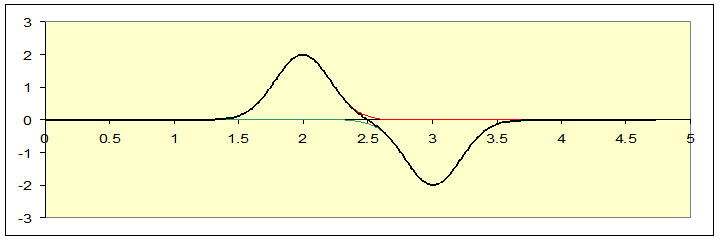
It’s easy to see that with this boundary condition, a pulse will be reflected without change of sign. Just take the spreadsheet and send down two pulses of the same sign:

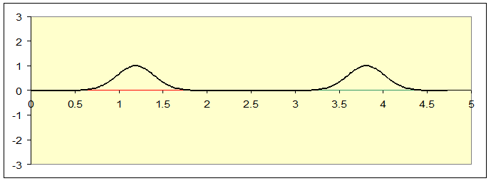
It’s evident from the complete symmetry that the slope of this curve is always going to be zero at the central point, so if we blind ourselves to the right-hand half, and imagine the left-hand half to be a complete string subject to the boundary condition at the right-hand end that the string slope be zero, a pulse coming towards the end from the left will be reflected without change of sign.

As mentioned earlier, although this is a rather artificial boundary condition for a string, we shall soon see it is exactly the right boundary condition for an open end of an organ pipe, so this analysis is relevant for some real-life systems.

The spreadsheet used to create the diagrams above is available here. After downloading (and clicking enable editing in the header strip) the waves can be animated by clicking and holding one end of the position slider bar.

There's also an applet animating the consequences of the different boundary conditions here.

previous index next