The One-Dimensional Random Walk

Michael Fowler

Flip a Coin, Take a Step

The one-dimensional random walk is constructed as follows:

You walk along a line, each pace being the same length.

Before each step, you flip a coin.

If it’s heads, you take one step forward. If it’s tails, you take one step back.

The coin is unbiased, so the chances of heads or tails are equal.

The problem is to find the probability of landing at a given spot after a given number of steps, and, in particular, to find how far away you are on average from where you started.

Why do we care about this game?

The random walk is central to statistical physics. It is essential in predicting how fast one gas will diffuse into another, how fast heat will spread in a solid, how big fluctuations in pressure will be in a small container, and many other statistical phenomena.

Einstein used the random walk to find the size of atoms from the Brownian motion.

The Probability of Landing at a Particular Place after n Steps

Let’s begin with walks of a few steps, each of unit length, and look for a pattern.

We define the probability function $f_{N} (n)$ as the probability that in a walk of $N$ steps of unit length, randomly forward or backward along the line, beginning at 0, we end at point $n .$

Since we have to end up somewhere, the sum of these probabilities over $n$ must equal 1.

We will only list nonzero probabilities.

For a walk of no steps, $f_{0} (0) = 1.$

For a walk of one step, $f_{1} (- 1) = \frac{1}{2}, f_{1} (1) = \frac{1}{2} .$

For a walk of two steps, $f_{2} (- 2) = \frac{1}{4}, f_{2} (0) = \frac{1}{2}, f_{2} (2) = \frac{1}{4} .$

It is perhaps helpful in figuring the probabilities to enumerate the coin flip sequences leading to a particular spot.

For a three-step walk, HHH will land at 3, HHT, HTH and THH will land at 1, and for the negative numbers just reverse H and T. There are a total of 2³ = 8 different three-step walks, so the probabilities of the different landing spots are: $f_{3} (- 3) = 1 / 8$ (just one walk), $f_{3} (- 1) = 3 / 8$ (three possible walks), $f_{3} (1) = 3 / 8, f_{3} (3) = 1 / 8.$

For a four-step walk, each configuration of H’s and T’s has a probability of ${(1 / 2)}^{4} = 1 / 16.$

So $f_{4} (4) = 1 / 16,$ since only one walk $—$ HHHH $—$ gets us there.

$f_{4} (2) = 1 / 4,$ four different walks, HHHT, HHTH, HTHH and THHH, end at 2.

$f_{4} (0) = 3 / 8,$ from HHTT, HTHT, THHT, THTH, TTHH and HTTH.

Probabilities and Pascal’s Triangle

If we factor out the $1 / 2^{N},$ there is a pattern in these probabilities:

n	-5	-4	-3	-2	-1	0	1	2	3	4	5
f₀(n)						1
2f₁(n)					1		1
2²f₂(n)				1		2		1
2³f₃(n)			1		3		3		1
2⁴f₄(n)		1		4		6		4		1
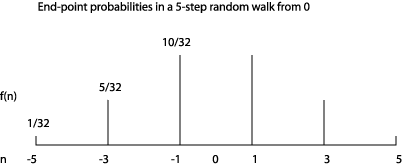
2⁵f₅(n)	1		5		10		10		5		1

This is Pascal’s Triangle $—$ every entry is the sum of the two diagonally above. These numbers are in fact the coefficients that appear in the binomial expansion of ${(a + b)}^{N} .$

For example, the row for $2^{5} f_{5} (n)$ mirrors the binomial coefficients:

${(a + b)}^{5} = a^{5} + 5 a^{4} b + 10 a^{3} b^{2} + 10 a^{2} b^{3} + 5 a b^{4} + b^{5} .$

To see how these binomial coefficients relate to our random walk, we write:

${(a + b)}^{5} = (a + b) \times (a + b) \times (a + b) \times (a + b) \times (a + b)$

and think of it as the sum of all products that can be written by choosing one term from each bracket. There are 2⁵ = 32 such terms (choosing one of two from each of the five brackets), so the coefficient of a³b² must be the number of these 32 terms which have just 3 a’s and 2 b’s.

But that is the same as the number of different sequences that can be written by rearranging HHHTT, so it is clear that the random walk probabilities and the binomial coefficients are the same sets of numbers (except that the probabilities must of course be divided by 32 so that they add up to one).

Finding the Probabilities Using the Factorial Function

The efficient way to calculate these coefficients is to use the factorial function. Suppose we have five distinct objects, A, B, C, D, E. How many different sequences can we find: ABCDE, ABDCE, BDCAE, etc.? Well, the first member of the sequence could be any of the five. The next is one of the remaining four, etc. So, the total number of different sequences is $5 \times 4 \times 3 \times 2 \times 1$ which is called “five factorial” and written 5!

But how many different sequences can we make with HHHTT? In other words, if we wrote down all 5! (that’s 120) of them, how many would really be different?

Since the two T’s are identical, we wouldn’t be able to tell apart sequences in which they had been switched, so that cuts us down from 120 sequences to 60. But the three H’s are also identical, and if they’d been different there would have been 3! = 6 different ways of arranging them. Since they are identical, all six ways come out the same, so we have to divide the 60 by 6, giving only 10 different sequences of 3 H’s and 2 T’s.

This same argument works for any number of H’s and T’s. The total number of different sequences of $m$ H’s and $n$ T’s is $(m + n)! / (m! n!)$ the two factorials in the denominator coming from the fact that rearranging the H’s among themselves, and the T’s among themselves, gives back the same sequence.

It is also worth mentioning that in the five-step walk ending at $-$ 1, which has probability 10/2⁵, the fourth step must have been either at 0 or $-$ 2. Glancing at Pascal’s Triangle, we see that the probability of a four-step walk ending at 0 is 6/2⁴, and of ending at $-$ 2 is 4/2⁴. In either case, the probability of the next step being to $-$ 1 is $½$ , so the total probability of reaching $-$ 1 in five steps is $½$ ×6/2⁴ + $½$ ×4/2⁴. So the property of Pascal’s triangle that every entry is the sum of the two diagonally above is consistent with our probabilities.

Picturing the Probability Distribution

It’s worth visualizing this probability distribution to get some feel for the random walk. For 5 steps, it looks like:

Let’s now consider a longer walk. After 100 steps, what is the probability of landing on the integer $n$ ?

This will happen if the number of forward steps exceeds the number of backward steps by $n$ (which could be a negative number).

That is,

$\begin{array}{l} n_{forward} - n_{backward} = n \\ n_{forward} + n_{backward} = 100 \end{array}$

from which

$n_{forward} = \frac{1}{2} (100 + n), n_{backward} = \frac{1}{2} (100 - n) .$

Note that in the general case, if the total number of steps $N$ is even, $n_{forward}, n_{backward}$ are both even or both odd, so $n,$ the difference between them, is even, and similarly odd $N$ means odd $n .$

The total number of paths ending at the particular point $n,$ from the heads and tails argument above, is

$\frac{100!}{(n_{forward})! (n_{backward})!} = \frac{100!}{(\frac{1}{2} (100 + n))! (\frac{1}{2} (100 - n))!} .$

To find the actual probability of ending at $n$ after 100 steps, we need to know what fraction of all possible paths end at $n .$ (Since the coin toss is purely random, we take it all possible paths are equally likely). The total number of possible 100-step walks is $2^{100} ≅ 1.26 \times 10^{30} .$

We’ve used Excel to plot the ratio: (number of paths ending at $n$ )/(total number of paths)

for paths of 100 random steps, and find:

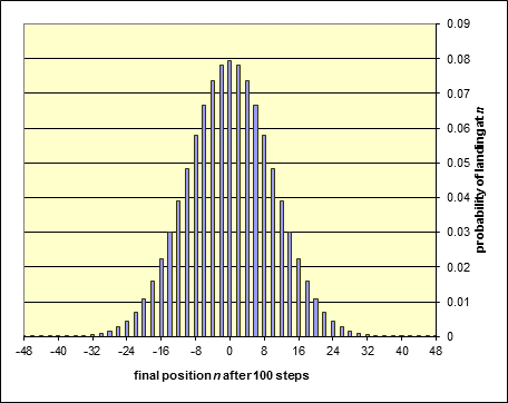
The actual probability of landing back at the origin turns out to be about 8%, as is (approximately) the probability of landing two steps to the left or right. The probability of landing at most ten steps from the beginning is better than 70%, that of landing more than twenty steps away well below 5%.

(Note: It’s easy to make this graph yourself using Excel. Just write -100 in A1, then =A1 + 2 in A2, then =(FACT(100))/(FACT(50 - A1/2)*FACT(50+A1/2))*2^-100 in B1, dragging to copy these formulae down to row 101. Then highlight the two columns, click ChartWizard, etc.)

It is also worth plotting this logarithmically, to get a clearer idea of how the probabilities are dropping off well away from the center.

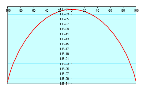
This looks a lot like a parabola $—$ and it is! Well, to be precise, the logarithm of the probability distribution tends to a parabola as $N$ becomes large, provided $n$ is much less than $N,$ and in fact this is the important limit in statistical physics.

The natural log of the probability of ending the path at $n$ tends to $\ln C - n^{2} / 200,$ where the constant $C$ is the probability $(100! / 50! 50!) / 2^{100}$ of ending the path exactly where it began.

This means that the probability $P (n)$ itself is given by:

$P (n) = C e^{- \frac{n^{2}}{200}}, C ≅ 0.08.$

This is called a Gaussian probability distribution. The important thing to notice is how rapidly it drops once the distance from the center of the distribution exceeds 10 or so. Dropping one vertical space is a factor of 100!

*Deriving the Result from Stirling’s Formula

(This more advanced material is not included in Physics 152.)

For large $N,$ the exponential dependence on $n^{2}$ can be derived mathematically using Stirling's formula $\ln n! ≅ n \ln n - n .$ That formula follows from

$\ln n! = \ln 1 + \ln 2 + \ln 3 + \dots + \ln n ≅ \int_{0}^{n} \ln x d x = {[x \ln x - x]}_{0}^{n} = n \ln n - n$ .

For a walk of $N$ steps, the total number of paths ending at $n$ is $\frac{N!}{(\frac{1}{2} (N + n))! (\frac{1}{2} (N - n))!} .$

To find the probability $P (n)$ we took one of these paths, we divide by the number of all possible paths, which is 2^N.

Applying Stirling’s formula

$\begin{matrix} \ln P (n) = \ln (\frac{N!}{(\frac{1}{2} (N + n))! (\frac{1}{2} (N - n))!} . \frac{1}{2^{N}}) \\ ≅ N \ln N - N - (\frac{N + n}{2}) \ln (\frac{N + n}{2}) + (\frac{N + n}{2}) - (\frac{N - n}{2}) \ln (\frac{N - n}{2}) + (\frac{N - n}{2}) - N \ln 2 \\ = N \ln N - (\frac{N + n}{2}) \ln (\frac{N + n}{2}) - (\frac{N - n}{2}) \ln (\frac{N - n}{2}) - N \ln 2 \end{matrix}$

then approximating

$\ln (\frac{N \pm n}{2}) = \ln \frac{N}{2} + \ln (1 \pm \frac{n}{N}) ≅ \ln \frac{N}{2} \pm \frac{n}{N} - \frac{1}{2} {(\frac{n}{N})}^{2}$

(using $\ln (1 \pm x) ≅ \pm x - x^{2} / 2$ for small $x$ ) the right-hand side becomes just $- n^{2} / 2 N .$

Actually, we can even get the multiplicative factor for the large $N$ limit ( $n$ much less than $N$ ) using a more accurate version of Stirling’s formula, $\ln n! ≅ n \ln n - n + \frac{1}{2} \ln 2 π n .$ This gives

$P (n) = \frac{2}{\sqrt{2 π N}} e^{- n^{2} / 2 N} .$

For $N = 100,$ this gives $P (0) = 0.08,$ P(0) = 0.08, within 1%, as we found with Excel. The normalization can be checked in the limit using the standard result for the Gaussian integral, remembering that $P (n)$ is only nonzero if $N - n$ is even.

So, How Far Away Should You Expect to Finish?

Since forward and backward steps are equally likely at all times, the expected average finishing position must be back at the origin. The interesting question is how far away from the origin, on average, we can expect to land, regardless of direction. To get rid of the direction, we compute the expected value of the square of the landing distance from the origin, the “mean square” distance, then take its square root. This is called the “root mean square” or rms distance.

For example, taking the probabilities for the five step walk from the figure above, and adding together +5 with $-$ 5, etc., we find the expectation value of $n^{2}$ is:

2 $\cdot$ 1/32 $\cdot$ 5² + 2 $\cdot$ 5/32 $\cdot$ 3² + 2 $\cdot$ 10/32 $\cdot$ 1² = 160/32 = 5.

That is, the rms distance from the origin after 5 steps is √5.

In fact,

The root mean square distance from the origin after a random walk of n unit steps is $\sqrt{n} .$

A neat way to prove this for any number of steps is to introduce the idea of a random variable. If $x_{1}$ is such a variable, it takes the value +1 or $-$ 1 with equal likelihood each time we check it. In other words, if you ask me “What’s the value of $x_{1}$ ?” I flip a coin, and reply “+1” if it’s heads, “ $-$ 1” if it’s tails. On the other hand, if you ask me “What’s the value of $x_{1}^{2}$ ?” I can immediately say “1” without bothering to flip a coin. We use brackets $〈 〉$ to denote averages (that is, expectation values) so $〈 x_{1} 〉 = 0,$ (for an unbiased coin), $〈 x_{1}^{2} 〉 = 1.$

The endpoint of a random walk of $n$ steps can be written as a sum of $n$ such variables:

Path endpoint = $x_{1} + x_{2} + \dots + x_{N} .$

The expectation value of the square of the path length is then:

$〈 {(x_{1} + x_{2} + \dots + x_{N})}^{2} 〉 .$

On squaring the term inside, we get $n^{2}$ terms. $n$ of these are like $〈 x_{1}^{2} 〉$ and so must equal 1. All the others are like $〈 x_{1} x_{2} 〉 .$ But this is the product of two different coin tosses, and has value +1 for HH and TT, $-$ 1 for HT and TH. Therefore it averages to zero, and so we can throw away all the terms having two different random variables. It follows that

$〈 {(x_{1} + x_{2} + \dots + x_{N})}^{2} 〉 = n .$

It follows that the rms deviation is $\sqrt{n}$ in the general case.

Density Fluctuations in a Small Volume of Gas

Suppose we have a small box containing $N$ molecules of gas. We assume any interaction between the molecules is negligible, they are bouncing around inside the box independently.

If at some instant we insert a partition down the exact middle of the box, we expect on average to find 50% of the molecules to be in the right-hand half of the box.

The question is: how close to 50%? How much deviation are we likely to see? Is 51% very unlikely?

Since the $N$ molecules are moving about the box in a random fashion, we can assign a random variable $y_{n}$ to each molecule, where $y_{n} = 1$ if the $n^{th}$ molecule is in the right hand half, $y_{n} = 0$ if the $n^{th}$ molecule is in the left-hand half of the box, and the values 1 and 0 are equally probable. The total number of molecules $N_{R}$ in the right-hand half of the box is then:

$N_{R} = y_{1} + y_{2} + \dots + y_{N} .$

This sum of $N$ random variables looks a lot like the random walk! In fact, the two are equivalent. Define a random variable $x_{n}$ by:

$y_{n} = \frac{1}{2} (1 + x_{n}) .$

Since $y_{n}$ takes the values 0 and 1 with equal probability, $x_{n}$ takes the values $-$ 1 and +1 with equal probability $—$ so $x_{n}$ is identical to our random walk one-step variable above. Therefore,

$N_{R} = y_{1} + y_{2} + \dots + y_{N} = \frac{1}{2} N + x_{1} + x_{2} + \dots + x_{N} .$

Evidently the sum of an $N$ -step random walk gives the deviation of the number of molecules in half the container from $N / 2.$ Therefore, from our random walk analysis above, the expectation value of this deviation is $\sqrt{N} .$ For example, if the container holds 100 molecules, we can expect a ten percent or so deviation at each measurement.

But what deviation in density can we expect to see in a container big enough to see, filled with air molecules at normal atmospheric pressure? Let’s take a cube with side 1 millimeter. This contains roughly 10¹⁶ molecules. Therefore, the number on the right hand side fluctuates in time by an amount of order $\sqrt{10^{16}} = 10^{8} .$ This is a pretty large number, but as a fraction of the total number, it’s only 1 part in 10⁸!

The probability of larger fluctuations is incredibly small. The probability of a deviation of $m$ from the average value $N / 2$ is:

$P (m) = C e^{- \frac{2 m^{2}}{N}} .$

So the probability of a fluctuation of 1 part in 10,000,000, which would be $10 \sqrt{N},$ is of order $e^{- 200},$ or about 10^-85. Checking the gas every trillionth of a second for the age of the universe wouldn’t get you close to seeing this happen. That is why, on the ordinary human scale, gases seem so smooth and continuous. The kinetic effects do not manifest themselves in observable density or pressure fluctuations $—$ one reason it took so long for the atomic theory to be widely accepted.

previous index next