To obtain our next equation of motion we appeal to Newton's Second Law--the mass of a fluid element times its acceleration is equal to the net force acting on that fluid element. If we take an element of unit volume, then we have
where ![]() is the force per unit volume on a fluid element. This
force may have several contributions. The first is the ``internal'' force
which is due to viscous dissipation, which we will ignore for right
now. The second set are ``body forces'' which act throughout the
volume of the fluid, such as the gravitational force. The third force
is due to pressure gradients within the fluid. To see how this works,
consider a cube of fluid, with dimensions
is the force per unit volume on a fluid element. This
force may have several contributions. The first is the ``internal'' force
which is due to viscous dissipation, which we will ignore for right
now. The second set are ``body forces'' which act throughout the
volume of the fluid, such as the gravitational force. The third force
is due to pressure gradients within the fluid. To see how this works,
consider a cube of fluid, with dimensions ![]() ,
, ![]() ,
and
,
and ![]() , as shown in Fig. 2.6.
, as shown in Fig. 2.6.
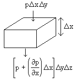
Figure 2.6: Derivation of the force on a fluid
element due to pressure gradients.
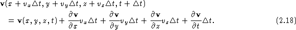
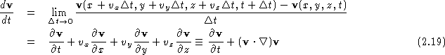
Now comes the tricky part. What is the acceleration of the
fluid? We want the acceleration of a particular element of the
fluid; the coordinates of this fluid element change in time as the
fluid flows. In a time interval ![]() , the x-coordinate
changes by
, the x-coordinate
changes by ![]() , the y-coordinate by
, the y-coordinate by ![]() ,
and the z-coordinate by
,
and the z-coordinate by ![]() . The velocity then
becomes
. The velocity then
becomes
To calculate the acceleration, we need to find the rate of change of the velocity:
We see that the acceleration is not simply
![]() . The reason for this is that even
if
. The reason for this is that even
if ![]() , so that the velocity at a
given point is not changing, that doesn't mean that a fluid element
is not accelerating. A good example is circular flow in a bucket.
If the flow is steady, then at a point in the bucket
, so that the velocity at a
given point is not changing, that doesn't mean that a fluid element
is not accelerating. A good example is circular flow in a bucket.
If the flow is steady, then at a point in the bucket
![]() , even though a fluid element in
the bucket is experiencing a centripetal acceleration. The term
, even though a fluid element in
the bucket is experiencing a centripetal acceleration. The term
![]() is nonlinear, and is the
source of all of the difficulties in fluid mechanics.
Pulling together all of the pieces, we have for our equation
of motion
is nonlinear, and is the
source of all of the difficulties in fluid mechanics.
Pulling together all of the pieces, we have for our equation
of motion
This is known as Euler's equationEuler's equation. This equation, along with the equation of continuity, are the governing equations of nonviscous fluid flow.
The Euler equation can be written in a somewhat different form which is often useful for applications. We use the following identity from vector calculus:
[see the PDR, p. 15, Eq. (12)]. Next we use
![]() , and the fact that
the fluid is incompressible so that
, and the fact that
the fluid is incompressible so that ![]() is constant, to rewrite
Eq. (2.20) as
is constant, to rewrite
Eq. (2.20) as