NUCLEAR MAGNETIC RESONANCE
Nuclear magnetic resonance (NMR) involves the interaction of a population
of nuclear spins in a d.c. magnetic field with an r.f. field at their precession
frequency. This frequency is given by
n = g(e/4pM)B
where g is the nuclear g-factor and M is the proton mass. For hydrogen
(i.e., protons), n/B = 4.26 MHz/Kilogauss, with
variations of several ppm depending on the local environment of the proton
(chemical shift). Thus for n = 30 MHz, B = 7.046
K Gauss. Pulsed NMR uses pulses of radio frequency magnetic fields of controlled
amplitude and duration to manipulate the nuclear spins in particular ways;
for instance, to rotate them by an angle of p or
p/2 from their initial direction of polarization.
The apparatus required for NMR consists of a magnet to produce a uniform
d.c. field H0, a small coil surrounding the spin-containing
sample to allow application of an r.f. magnetic field H1, and
another (or the same) coil to pick up the induced magnetic flux produced
by the precessing spins. The electronic components described here allow
the generation of suitable r.f. pulses and the detection of the induced
flux.
Setup:
Magnet power supply - Harvey-Wells Magnet with Walker Scientific Power
Supply
-
Turn on water to magnet ~50% (Don't forget - there is no interlock
protection). Monitor that exiting water becomes neither very warm nor so
cold as to induce condensation.
-
Turn "power" on (switch on left.)
-
[IMPORTANT] Set "current adjust"
"coarse" to 0 and "fine" at midrange.
-
[IMPORTANT] Wait 60 sec. Then
push "dc on" button.
-
Turn "current adjust" "coarse" to LED readout of 80.2 (this
number is "% of max" and gives about 7kG, as required for proton resonance
at 30 MHz.)
-
Search for resonance using "current adjust, coarse" very slowly
in the range 80.0 - 80.5 with r.f. pulses set as described below and observing
the output signal on the scope.
-
Use single pulse "A", approximately 10 µs long; Power Amplifier gain
~1/5 of knob range (horizontal, left)
-
Scope sweep 10 or 20 µs/div. Watch just to the right of the pulse.
-
Probe in the center of the magnet.
-
Mineral oil or dirty water sample in the probe.
Shut down:
-
[IMPORTANT] Turn
"course current" adjust to 0.
-
When current = 0, push "dc off" button. [VERY
IMPORTANT to do step 2 before 3!]
-
Turn off power switch.
-
Turn off water.
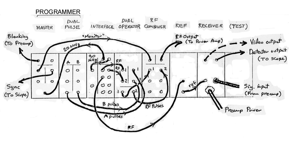
Spectrometer: Digital Timing Panels
| R: 100 × 103 ms
R |
Recurrent Sync |
|
| L: 50 × 103 ms
R |
|
|
|
|
|
| A: 202 × 100 ms
R |
Analog |
1-10 µs |
| B: 101 × 100 ms
R |
Analog |
1-10 µs |
Modules
| Programmer, Master |
Blanking = 1 turn CW |
| Pulse Gen |
A = 1 - 10 ms
B = 1 - 10 ms |
|
|
0o/90o |
0o/180o |
Coarse. Don't change unless necessary |
| Operator |
Ch1 = f
Ch2 = f |
0o
0o |
0o
0o |
CCW+3tCW
CCW+3tCW |
|
Att. 0 db |
|
|
|
| Rf Combiner |
Att. 0 db |
|
|
CCW |
| Ref |
|
0o |
180o |
CCW |
| Receiver |
5ms, Att.12db |
|
|
CCW+3tCW |
Procedure:
Turn on the power amplifier, with gain set 1/5 turn from minimum (min.
= fully CCW). Make sure the sample tube is filled to 5-7 mm and the sample
is centered axially in the coil, using the mark on the outside of the probe
cover. Assume the probe is already tuned (see elsewhere for tuning procedure).
Monitor the "detected output" from the receiver on the oscilloscope,
using about 1 ms/div and enough gain to see just a little noise. Adjust
the magnetic current slightly to find the resonance. When you find something,
adjust the current a little farther to make sure it is not a sideband (due
to gating r.f. into pulses). Fine adjust the magnet current to maximize
the period of the beat between the free precision and the 30 MHz reference.
After the magnet drift has decreased to a reasonable rate, engage the flux
stabilization circuit (see below).
Set up a p-pulse: (Channel A -> 1)
Start with the analog pulse width vernier fully CCW (1 ms).
Turn CW until the initial amplitude of the free induction decay (FID) signal
is maximum and continue until it decreases to zero. You may have to go
to the 10-100 ms range, but start on 1-10 ms
to be sure you get the first zero. Connect the scope to an unused "pulse
output" jack on module "B" and measure the pulse width.
Set up a p/2-pulse: (Channel b ->2)
(1) Adjust for the (first) maximum initial FID amplitude; or better:
(2) set width to half that of a p-pulse. For
more precise setting, use the multiple pulse procedure described later.
Set phase adjustments:
Since only relative phases matter, the three sets of phase controls
(Channel 1, Channel 2, and reference) are redundant. Therefore leave the
Channel 1 settings fixed (unless it is convenient to introduce a 90o
or 180o shift there; but leave the continuous adjustments fixed
in any case). With an approximately p/2 pulse
from Channel A/Channel 1, adjust the reference phase to maximize the initial
amplitude of the FID. [NOTE: Due to a bad relay, the channel
1 switch "0/90 deg" should be left on 0 deg. Change the phase of
the receiver instead.]
Standard pulse sequences
Initial reading:
-
Slichter, 2nd edition, pp. 1-42, especially classical sections, especially
pp. 1-10 and 38-42.
-
Fukushima and Roeder, pp. 1-35, especially pp. 25-35.
-
Gerstein and Dybowski, (Reference for pulse sequences).
The quantities which can be determined in NMR are the number of spins of
a particular type (~strength of signal); the chemical shift (i.e., the
exact magnetogyric ratio); and the longitudinal (T1) and transverse
(T2) relaxation times. These relaxation times were introduced
by Bloch (Phys. Rev. 70, 460 (1946); see also Slichter or most any
textbook). T1 is the characteristic time for recovery of the
magnetization along the static field to its thermal equilibrium value.
T2 is the intrinsic time constant for decay of a transverse
magnetization which is precessing around the static field (in the x - y
plane); this relaxation may be enhanced by processes, such as dipole-dipole
coupling between spins, which do not contribute to T1. Finally,
T2* describes the non-intrinsic decay of a transverse magnetization
due to inhomogeneity of the static field: spins at different positions
in the sample will precess at different rates, and soon they will average
to zero. We will be mostly concerned with measuring these relaxation times.
(1) Single p/2-pulse (or any pulse length
not equal to np):
This will tilt the magnetization rom the z-direction to the y-direction
(for a p/2-pulse with H1 in the x-direction)
or in general will tilt some component into the x - y plane, where it will
precess, and this precessing magnetization can be picked up by the receiver.
Its magnitude will decay at a rate 1/Tm = 1/T2 +
1/T2*. For a liquid sample normally T2 >> T2*,
so Tm @ T2*.
(2) Sequence p, delay t,
p/2:
The initial p-pulse tilts the magnetization
from the +z to the -z direction (from an energy level point of view, it
inverts the population of the nuclear Zeeman levels). The magnetization
then relaxes towards equilibrium (+z) with time constant T1.
So far we see nothing because only magnetization precessing in the x -
y plane can be detected. The p/2 pulse after
delay tilts whatever z-magnetization Mz (t)
exists at that time, whether negative or positive, into the y-direction.
This gives a signal whose initial magnitude is proportional to Mz
(t). The experiment is repeated for different
values of t and compared to the predicted relation:
Mz(t) = M0[1 -
2exp(-t/T1)]
to obtain T1. Note that Mz (t)
= 0 at = T1ln2.
(3) Sequence (p/2)x, delay t,
px (spin echo):
The p/2 pulse tilts the magnetization to
the y axis in the rotating frame. It then fans out in the x - y plane during
the period due to inhomogeneity of H0. The p
rotates each spin 180o around the x axis. Each spin then
continues to precess at the same rate as before. Consequently, regardless
of its precession rate, it reaches the - y axis after an addition time
t. This gives the "echo" or "refocusing."
The half-width of the echo pulse is characterized by T2*. The
decay of the echo amplitude as a function of delay 2t
is determined by T2.
Now some extended pulse sequences:
(4) Flip-flop sequence, [(p/2)x ,
t]n:
This is a sequence of identical p/2 pulses
at interval t. If the pulses are in fact exactly
p/2, then after any even number of pulses the
magnetization should be in the ±z direction and the output zero.
This is illustrated in Gerstein and Dybowski, p. 176, Figs. 5-6 and 5-7.
Figure 5-8 shows what happens if the sample is too large: H1
is then not uniform over the whole sample, and the pulse strength cannot
be p/2 for all parts. This sequence can be used
to trim the pulse length to p/2.
(5) Alternated-phase flip-flop sequence [(p/2)x
, t , (p/2)-x
, t]n:
In this sequence, alternate p/2 pulses are
phase-shifted by 180o, i.e. the sign of H1 is reversed
for alternate pulses. Thus the magnetization is tilted from z to y and
then back to z. If the x pulses (generated by Channel A, say, with fA
= 0o) and the -x pulses (generated by Channel B with fB
= 180o) are both exactly p/2 in strength
but are not exactly 180o out of phase, then there will be a
cumulative error in returning the magnetization to the z direction, which
will modulate the signal envelope. This can be used to set the phase of
Channel B relative to Channel A
(6) Carr-Purcell sequence: (p/2)x ,
t , [px , t]n:
This is a "spin-echo" technique, used to measure T2. The
effect of inhomogeneity of H0, which causes the FID to decay
with time constant T2* << t <
T2. In this sequence it is critical that the p
pulses be exactly p, otherwise the magnetization
will develop a cumulative tilt out of the x - y plane, and the apparent
decay time will be less than T2.
(7) Carr-Purcell-Meiboom-Gill (CPMG) sequence: (p/2)x
, t , [py , 2t]n:
This differs from the Carr-Purcell sequence only in that the p
pulses are phase shifted 90o relative to the p/2
pulse. This means that the spins fanning out from the y- axis are rotated
180o about the y (instead of x) axis to set up the echoes. See
F & R, p. 32 and G & D, p. 193 ff, especially Fig. 5-15. The advantage
of this is that a p pulse width error does not
have a cumulative effect, and in fact cancels out for even-numbered echoes
(see G & D, Fig. 5-16).
(The width of the p-pulse could be adjusted
to the correct value by observing in the CPMG sequence when the odd echoes
fall on the same exponential decay envelope as the even echoes, or in the
CP sequence by maximizing the decay time.)
(8) Waugh-Huber-Haeberlen (WAHUHA) sequence:
This is a four-pulse cycle which suppresses the effect of dipole-dipole
interactions. We cannot do it at U.Va. because it requires two dual pulse
generators.
Experiments:
-
Find the resonance in "dirty"* water and observe FID. (* dilute solution
of NiCl, barely yellow, to reduce T1 to a reasonable value.)
Or use mineral oil.
-
Setup p and p/2 pulses
and study various pulse sequences qualitatively, getting rough delay times.
-
Measure T2*, T2, and T1 by one or more
methods and try to understand any differences in values for different methods.
-
See effect of different impurity concentrations in the water; look at protons
in mineral oil or possibly methanol.
-
Possibly look at 19F in a compound such as CCl2F2
(freon).
Probe
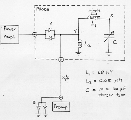
-
L1: 18 turns of 0.7 mm diameter wire on 9.0 mm OD glass tube,
approximately 15mm long.
-
L2: 4 turns on Bakelite (non-magnetic) toroid.
Front Panel Coax Connections