Functions of a Complex Variable: Contour Integration and Steepest Descent
Michael Fowler
Analytic Functions
Suppose we have a complex function of a complex variable defined in some region of the complex plane, where are real. That is to say,
with and real functions in the plane.
We now assume that in this region is differentiable, that is to say,
is well-defined. What does this tell us about the functions and the real and imaginary parts of ?
In fact, the property of differentiability for a function of a complex variable tells us a lot! It does not just mean that the function is reasonably smooth. The crucial difference from a function of a real variable is that can approach zero from any direction in the complex plane, and the limit in these different directions must be the same. Of course, there are only two independent directions, so what we are really saying is
which we can write in terms of
Equating real and imaginary parts of this equation we find:
These are called the Cauchy-Riemann equations.
It immediately follows that both and must satisfy the two-dimensional Laplacian equation,
that is,
Notice that this implies (just as for an electrostatic potential) that cannot have an absolute minimum or maximum inside the region of analyticity. If but the second-order partial derivatives are nonzero, then they must have opposite sign, signaling a saddlepoint. In the general case, a two-dimensional version of Gauss’ theorem can be used to show there is no local extremum.
Furthermore,
That is to say, the contour lines of constant are everywhere orthogonal to the contour lines of constant (The gradient being orthogonal to the contour lines everywhere.)
The important point is that just requiring differentiability of a function of a complex variable imposes a strong constraint on its real and imaginary parts, the functions and
A Simple Example: f (z) = z2.
It is worthwhile building a clear picture of the real and imaginary parts of the function The real part is and its contour lines in the square −1 to 1 are shown below. The darker shades are the lower ground. At the origin, there is a saddlepoint with higher ground in both directions of the real axis, lower ground in the pure imaginary directions. The lines (not shown) are contours at the same level (zero) as the origin.
What about the imaginary part? has contours:
Putting the two sets of contour lines on the same diagram it is clear that they always cut each other orthogonally:
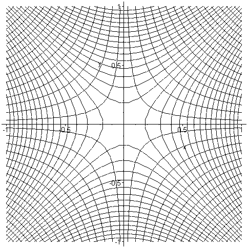
(Incidentally, this picture has a physical realization. It represents the field lines and equipotentials of a quadrupole magnet, used for focusing beams of charged particles.)
Another Example: f(z) = 1/z
The definition of differentiation above can be used to show that
just as for a real variable, so the function can be differentiated everywhere in the complex plane except at the origin. The singularity at the origin is termed a “pole”, for obvious reasons.
Contour Integration: Cauchy’s Theorem
Cauchy’s theorem states that the integral of a function of a complex variable around a closed contour in the complex plane is zero if the function is analytic in the region enclosed by the contour.
This theorem can be proved at various levels of rigor (see Byron and Fuller for details), we shall give a basic physicist’s proof using Stokes theorem, that the integral of a vector function around a contour (now in ordinary, not complex, space) is equal to the integral of the curl of that function over an area spanning the contour, provided of course the curl is well-defined everywhere on the area,
Taking the special case where the contour and the area are confined to the plane, and writing , , and Stokes’ theorem becomes:
known in this form as Green’s theorem (and easy to prove: the two terms are separately equal, , this can be established by dividing the area into strips of infinitesimal width parallel to the -axis, integrating with respect to within a strip, to give , the co-ordinates of the points on the contour at the ends of the strip, then adding the contributions from all the parallel strips just gives the integral around the contour.)
Now back to the complex plane: write as before
from which
Now apply Green’s theorem to the two integrals on the right, replacing with first then with This gives:
and both these integrals are identically zero from the Cauchy-Riemann equations.
So the integral of a function of a complex variable around a closed contour in the complex plane can only depend on nonanalytic behavior inside the contour. Consider for example a pole, take the simplest case of integrating around the unit circle, the conventional direction is counterclockwise. Then ,
This is called the residue at the pole.
Moving the Contour of Integration
Cauchy’s theorem has a very important consequence: for an integral from, say, to in the complex plane, moving the contour in a region where the function is analytic will not affect the result, because the difference between the integral over the original contour and that over the shifted contour is an integral around a closed circuit, and therefore zero, provided the function is analytic in the region enclosed.
For an integral around a closed contour, if the only singularities enclosed by the contour are poles, the contour may be shrunk and broken to become a sum of separate small contours, one around each pole, then the integral around the original contour is the sum of the residues at the poles.
Other Singularities: Cuts, Sheets, etc.
Poles are of course not the only possible singularities. For example, has a singularity at the origin. Now, The singularity at the origin is from the term, but notice that if we go around the unit circle, increases by and if we go around again it increases by a further This means that the value of is not uniquely defined: any given point in the complex plane has values differing by any integer. This is handled by replacing the single complex plane with a pile of sheets, and a cut going out from the origin. To find you need to know not only but also which sheet you’re on: going up one sheet means has increased by When you cross the cut, you go to the next sheet, like a multilevel parking garage. The cut can go out from the origin in any direction, the standard arrangement is along the real axis, either positive or negative.
The square root function similarly has a cut, but only two sheets.
Evaluating Rapidly Oscillating Integrals by Steepest Descent
How to evaluate in an unambiguous fashion: an introduction to moving the contour of integration and the Method of Steepest Descent.
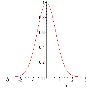
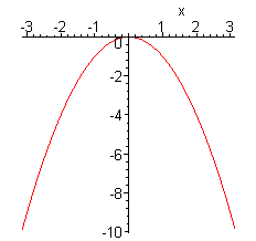
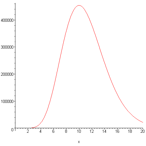
The familiar Gaussian integral is easy to understand. Plotting the integrand, (here for ) there is a peak of height 1 and width of order
But what about the result ? This (correct) result is far less obvious! Here the integrand is always on the unit circle in the complex plane, and equal to 1 at It is instructive to plot the phase of the integrand as a function of (taking in the graph below).
The phase is stationary at the origin, so contributions from that region add coherently. To help visualize the integrand better, here’s a plot of the real part:
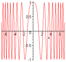
It is evident that almost all the contribution to the integral comes from the central region where the phase is stationary, the increasingly rapid oscillations away from the origin ensuring that very little comes from elsewhere.
So how do we actually evaluate the integral? In the complex plane we can write
Notice that the amplitude (or modulus) of the integrand is always unity on the real axis, so it does not go to zero at infinity, although there are essentially no contributions from large because of the rapid oscillations.
A cleaner way to see what’s going on is to rotate the contour of integration around the origin to the 45 degree line It’s safe to do this because the amplitude of the integrand decreases on going from the real axis into the region and in fact tends to zero on going to infinity in that region.
(To give a more precise argument, suppose we replace the infinite integral by one from to so we will be taking the limit of going to infinity at the end. Then the distorted contour has first a vertical part, from to then the diagonal contour from to finally another vertical leg from to Now, on the first vertical part, the integral is clearly less than the integral of the modulus, that is,
with so
the required result.
General Steepest Descent Method
In fact, the contour rotation trick used above to make the integral easier to evaluate is a particular case of a method having wide applicability in evaluating contour integrals of the form . The basic strategy is to distort the contour of integration in the complex -plane so that the amplitude of the integrand is as small as possible over as much of the contour of integration as possible. Actually, that is exactly what we did in the example above. To see this, it is helpful to plot the contour lines (lines of constant value) of the modulus of the integrand,
The convention here is white for the high ground, black for the valleys.
We want to keep the contour of integration as low as possible for as long as possible. The map above is of a “saddlepoint”: hills rise to the northeast and the southwest of the origin, valleys fall away to the northwest and the southeast. The strategy is to stay in the valleys (small integrand) as much as possible -- however, to get from to we have to get from one valley to the other, and that means going over the saddlepoint at the origin. Obviously, to get the integrand as small as possible at all stages in the integration we must go down from the saddlepoint in both directions by the steepest possible route, and it is evident that this is right down the center of the valley, just the contour we chose above. Note that this steepest descent path is also one of stationary phase. This is because for any analytic function of a complex variable the lines of constant are perpendicular to those of constant For a function , the steepest descent line is perpendicular to the lines of constant and is therefore a line of constant that is, constant phase of .
Saddlepoints of Analytic Functions
Suppose we have a function analytic in some region of the complex plane, and at some point inside the derivative Then in the neighborhood of
Close enough to we can neglect the higher order terms, and for the case of real, the contour lines of the real and imaginary parts of will then be exactly those we have plotted for above. For complex, the plots will be rotated by an angle equal to the phase of
That is to say, for any analytic function, near any point where (and nonzero second derivative) the real and imaginary parts of the function have saddlepoints with contour maps rotated versions of those above.
Integrating Through a Saddlepoint
We consider now integrals of the form
where is some path in a region where is analytic. This means the value of the integral will not be affected by distorting the path, provided it stays in the region of analyticity. (The path of integration is usually called the contour of integration -- we’ll call it path here, to avoid confusion with our contours, which have the standard geographic meaning, joining points having the same value of some parameter.)
Note that with the exponential form of the integrand, the real part of determines the magnitude of the integrand, the imaginary part of determines its phase.
The strategy is to arrange the path of integration so that as much as possible of it is in the valleys, where the integrand is small, then to go over the saddlepoint by the steepest possible route, which would be staying on the imaginary axis in the case of plotted above. It is important to note that this “steepest descent” route is also a path along which the imaginary part of remains constant, so the contributions along this path are all in phase, that is to say, they add coherently.
The bottom line is that by directing the path of integration through the saddlepoint along the steepest route for the magnitude of the integrand, the biggest contributions to the integral are all in phase. Along this path, the integral has standard Gaussian form. If the function is sufficiently large, it may be that the contribution of the integral away from the saddlepoint can be neglected. This method is therefore often valuable in cases where some parameter becomes large: we give a number of examples to clarify this point.
Saddlepoint Estimation of n!
We use the identity
here it is for
Note that
Therefore, in the neighborhood of the maximum value of at
For integer the function is analytic in any finite region of the complex plane. Taking as in the real-axis graph above, and plotting the contours of in the neighborhood of we find:
It is clear that the integral along the real axis is in fact a steepest descent path. The reason we look at this straightforward case is to gain some experience about when it is reasonable to throw away all the contribution to the integral except that near the saddlepoint. If we simply take
and take the integration to be over the whole real axis, not just positive it is a Gaussian integral and
More precise, and considerably more complicated, methods give the leading correction to this expression. It is down by a factor of so the naïve Gaussian saddlepoint result is accurate within 1% for and improves as increases.
The Delta Function
Recall that the delta function can be defined by the limit of a Gaussian integral
It is easy to see how this leads to
for an integral along the real axis with a function reasonably well-behaved near the origin. Shankar mentions that the definition also works even if is replaced by . In that case, the absolute value of the function is the same everywhere on the real axis, and increases as on taking small. The reason it still works is that the phase oscillations are so rapid everywhere except at the origin, where the phase is momentarily stationary, so all the contribution comes from there.
This is just revisiting our earlier discussion of the Gaussian integral (apart from a trivial change of sign). And, as before, the way to evaluate the integral
is to rotate the integration contour by about the origin into the complex plane. That is, change the variable of integration from to where The integral becomes a simple real Gaussian. The steepest descent route through the origin is now along the line at to the real axis. So this is a perfectly good definition of the -function provided we can distort the path of integration from the real axis to the line (Strictly speaking, the path would now include two octants of a circle at very large -- their contribution vanishes in the limit of going to infinity.)
previous home next PDF