Adding Angular Momenta

Michael Fowler, UVa.

Introduction

Consider a system having two angular momenta, for example an electron in a hydrogen atom having both orbital angular momentum and spin. The ket space for a single angular momentum has an orthonormal basis $| j, m 〉$ so for two angular momenta an obvious orthonormal basis is the set of direct product kets $| j_{1}, m_{1} 〉 \otimes | j_{2}, m_{2} 〉 .$ What does this mean, exactly? Suppose the first angular momentum ${\vec{J}}_{1}$ has magnitude ${\vec{J}}_{1}^{2} = ℏ^{2} j_{1} (j_{1} + 1)$ , and is in the state $\sum_{m_{1} = - j_{1}}^{j_{1}} α_{m_{1}} | j_{1}, m_{1} 〉$ , and similarly the second angular momentum ${\vec{J}}_{2}$ is in the state $\sum_{m_{2} = - j_{2}}^{j_{2}} β_{m_{2}} | j_{2}, m_{2} 〉$ . Evidently the probability amplitude for finding the first spin in state $m_{1}$ and at the same time the second in $m_{2}$ is $α_{m_{1}} β_{m_{2}},$ and we denote that state by $| j_{1}, m_{1} 〉 \otimes | j_{2}, m_{2} 〉 .$ How to handle these direct product spaces will become clear on examining specific examples, as we do below, beginning with two spins one-half.

Now the sum of two angular momenta $\vec{J} = {\vec{J}}_{1} + {\vec{J}}_{2}$ is itself an angular momentum, operating in a space with a complete basis $| j, m 〉 .$ This is easy to prove: the components of ${\vec{J}}_{1}$ satisfy $[J_{1 i}, J_{1 j}] = i ℏ ε_{i j k} J_{1 k}$ , and similarly for the components of ${\vec{J}}_{2}$ . The components of ${\vec{J}}_{1}$ commute with the components of ${\vec{J}}_{2}$ , of course, from which it follows immediately that the vector components of $\vec{J} = {\vec{J}}_{1} + {\vec{J}}_{2}$ do indeed obey the angular momentum commutation relations: and recall that the commutation relations were sufficient to determine the allowed sets of eigenvalues. We shall prove later that the eigenstates $| j, m 〉$ of ${\vec{J}}^{2}, {\vec{J}}_{z}$ are a complete basis for the product space of the eigenkets of ${\vec{J}}_{1}^{2}, {\vec{J}}_{2}^{2}, J_{1 z}, J_{2 z}$ $—$ to establish this, we must first find the possible allowed values of the total angular momentum quantum number $j .$

Here we have, then, two different orthonormal bases for what is evidently the same vector space. In practical applications, it often turns out that we have to translate from one of these bases to the other. Our present task is to construct the appropriate transformation: we accomplish this by finding the coefficients of any $| j, m 〉$ in the $| j_{1}, m_{1} 〉 \otimes | j_{2}, m_{2} 〉$ basis. (These are called the Clebsch-Gordan coefficients.)

We shall build gradually, beginning with adding two spins one-half, then a spin one-half with an orbital angular momentum, finally two general angular momenta.

Adding Two Spins: the Basis States and Spin Operators

The most elementary example of a system having two angular momenta is the hydrogen atom in its ground state. The orbital angular momentum is zero, the electron has spin angular momentum $\frac{1}{2} ℏ$ , and the proton has spin $\frac{1}{2} ℏ$ .

The space of possible states of the electron spin has the two basis kets ${| ↑ 〉}_{e} and {| ↓ 〉}_{e}$ , (also variously written as $| + 〉, | - 〉; (\begin{matrix} 1 \\ 0 \end{matrix}), (\begin{matrix} 0 \\ 1 \end{matrix}); χ_{+}, χ_{-}$ !) the basis proton spin kets are ${| ↑ 〉}_{p} and {| ↓ 〉}_{p}$ , so the possible states of the combined system are kets in the direct product space which has a basis of four kets:

$| ↑_{e} ↑_{p} 〉, | ↑_{e} ↓_{p} 〉, | ↓_{e} ↑_{p} 〉, | ↓_{e} ↓_{p} 〉$

using $| ↑_{e} ↑_{p} 〉$ as shorthand for ${| ↑ 〉}_{e} \otimes {| ↑ 〉}_{p}$ .

Note here that we’ve written the kets in “alphabetical order” with $↑$ as the first letter, $↓$ as the second. That is to say, we’ve first written all the kets having $↑$ as the first letter, etc.

For the more general case of adding $j_{1}$ to $j_{2},$ to be considered shortly, we’ll order the kets in the same “alphabetical” way, writing first all the kets having $m_{1} = j_{1},$ and so on down to $m_{1} = - j_{1} :$

$(j_{1} j_{2}, j_{1} (j_{2} - 1), \dots, j_{1} (- j_{2}), (j_{1} - 1) j_{2}, (j_{1} - 1) (j_{2} - 1), \dots, (j_{1} - 1) (- j_{2}), \dots, (- j_{1}) (- j_{2})) .$

The dimensionality of this space is then $(2 j_{1} + 1) \times (2 j_{2} + 1) .$

Now the first block of $2 j_{2} + 1$ elements all have the same $m -$ component of $j_{1},$ that is, $m_{1} = j_{1},$ the next block has $m_{1} = j_{1} - 1,$ and so on. Think about what this means for constructing a rotation operator acting on the kets in this space: if it operates only on the angular momentum $j_{1},$ it will change the factors $m_{1}$ multiplying the blocks, if the operator rotates only $j_{2},$ it will operate within each block, all the blocks being changed in the same way.

To get a feeling for how this works in practice, we go back to the simplest case, two spins one-half.

The space is four-dimensional, having basis $| ↑_{e} ↑_{p} 〉, | ↑_{e} ↓_{p} 〉, | ↓_{e} ↑_{p} 〉, | ↓_{e} ↓_{p} 〉$ .

Any operator acting on the spins will be represented by a $4 \times 4$ matrix, best thought of as a $2 \times 2$ matrix made up of $2 \times 2$ blocks: an operator acting on the proton spin acts within the blocks, one operating on the electron spin affects the overall multiplying factors in front of each block.

Let’s look at a few examples. Recall that the raising operator for a single spin is the $2 \times 2$ matrix $S^{+} = ℏ (\begin{matrix} 0 & 1 \\ 0 & 0 \end{matrix}) .$ So what is the raising operator for the electron spin?

$S_{e}^{+} \otimes I_{p} = ℏ (\begin{matrix} 0 & I \\ 0 & 0 \end{matrix}) = ℏ (\begin{matrix} 0 & 0 & 1 & 0 \\ 0 & 0 & 0 & 1 \\ 0 & 0 & 0 & 0 \\ 0 & 0 & 0 & 0 \end{matrix}) .$

We use bold to denote $2 \times 2$ matrices.

The pattern is clear: the big structure (in bold above), that of the four 2×2 blocks, reflect the structure of the electron spin operator $S^{+} = ℏ (\begin{matrix} 0 & 1 \\ 0 & 0 \end{matrix}),$ within those blocks (of which only one survives) the identity operator $I = (\begin{matrix} 1 & 0 \\ 0 & 1 \end{matrix})$ acts on the proton spin.

The operator that raises the proton spin is:

$I_{e} \otimes S_{p}^{+} = ℏ (\begin{matrix} σ^{+} & 0 \\ 0 & σ^{+} \end{matrix}) = ℏ (\begin{matrix} 0 & 1 & 0 & 0 \\ 0 & 0 & 0 & 0 \\ 0 & 0 & 0 & 1 \\ 0 & 0 & 0 & 0 \end{matrix}) .$

What about the operator that raises both electron and proton spin? In this case, the pattern of blocks, and the pattern within each block, must both be $(\begin{matrix} 0 & 1 \\ 0 & 0 \end{matrix})$ , so

$S_{e}^{+} \otimes S_{p}^{+} = ℏ^{2} (\begin{matrix} 0 & σ^{+} \\ 0 & 0 \end{matrix}) = ℏ^{2} (\begin{matrix} 0 & 0 & 0 & 1 \\ 0 & 0 & 0 & 0 \\ 0 & 0 & 0 & 0 \\ 0 & 0 & 0 & 0 \end{matrix}) .$

There is only one nonzero matrix element because only one member of the base survives this operation.

If two spins interact (via their magnetic moments, for example) in a way that preserves total angular momentum, a possible term in the Hamiltonian would be $S_{e}^{-} S_{p}^{+},$ represented by:

$S_{e}^{-} S_{p}^{+} = ℏ (\begin{matrix} 0 & 0 & 0 & 0 \\ 0 & 0 & 0 & 0 \\ 0 & 1 & 0 & 0 \\ 0 & 0 & 0 & 0 \end{matrix}) = ℏ S_{e}^{-} \otimes S_{p}^{+} .$

Representing the Rotation Operator for Two Spins

Recall from the lecture on spin that the rotation operator on a single spin one-half is

$D^{(1 / 2)} (R (θ \hat{\vec{n}})) = e^{- \frac{i θ \hat{\vec{n}} \cdot \vec{J}}{ℏ}} = e^{- i (θ / 2) (\hat{\vec{n}} \cdot \vec{σ})} = I \cos \frac{θ}{2} - i (\hat{\vec{n}} \cdot \vec{σ}) \sin \frac{θ}{2}$

in the $2 \times 2$ spinor space. As we established, this matrix operator has the form

$(\begin{matrix} a & b \\ - b^{*} & a^{*} \end{matrix}) = (\begin{matrix} \cos (θ / 2) - i n_{z} \sin (θ / 2) & - (i n_{x} + n_{y}) \sin (θ / 2) \\ (- i n_{x} + n_{y}) \sin (θ / 2) & \cos (θ / 2) + i n_{z} \sin (θ / 2) \end{matrix}) .$

with ${| a |}^{2} + {| b |}^{2} = 1.$

This set of unitary $2 \times 2$ matrices form a representation of the rotation group in the sense that the total resulting from two successive rotations is given by the matrix which is the matrix product of those corresponding to the two rotations.

From the discussion in the previous section, it should be clear that in the product space of the two spins, the representation of the rotation operator $—$ both spins of course undergoing the same rotation $—$ is:

$(\begin{matrix} a (\begin{matrix} a & b \\ - b^{*} & a^{*} \end{matrix}) & b (\begin{matrix} a & b \\ - b^{*} & a^{*} \end{matrix}) \\ - b^{*} (\begin{matrix} a & b \\ - b^{*} & a^{*} \end{matrix}) & a^{*} (\begin{matrix} a & b \\ - b^{*} & a^{*} \end{matrix}) \end{matrix}) = (\begin{matrix} a^{2} & a b & a b & b^{2} \\ - a b^{*} & a a^{*} & - b b^{*} & a^{*} b \\ - a b^{*} & - b b^{*} & a a^{*} & a^{*} b \\ b^{* 2} & - a^{*} b^{*} & - a^{*} b^{*} & a^{* 2} \end{matrix}) .$

This set of $4 \times 4$ matrices, again with ${| a |}^{2} + {| b |}^{2} = 1,$ must also form a representation of the rotation group over the four-dimensional space. We shall shortly discover that this representation can be simplified, but to achieve that we need to analyze the states in terms of total angular momentum.

Representing States of Two Spins in Terms of Total Angular Momentum

We’re now ready to look at total spin states for the ground-state (zero orbital angular momentum) hydrogen atom.

Consider first the state with both electron and proton spin pointing upwards, $| ↑ ↑ 〉$ . The $z -$ component of the total spin is $S_{z} = S_{z}^{e} + S_{z}^{p}$ , so $S_{z} = ℏ$ . Labeling the total spin state $| s, m 〉$ , we have a state with $m = 1,$ so $s = 1.$ (To confirm that this state indeed has $s = 1$ we can apply the total-spin raising operator $S_{+} = S_{+}^{e} + S_{+}^{p}$ . Since both component spins have maximum $m$ value, $S_{+} {| s, 1 〉}_{s m} = (S_{+}^{e} + S_{+}^{p}) | ↑ ↑ 〉 = 0$ , but $S_{+}$ only gives zero when acting on the $m = s$ member of a multiplet. )

We find, then, that $| ↑ ↑ 〉 = {| 1, 1 〉}_{s m}$ where we’ve added the suffix $s m$ to make clear that the numbers in the last ket signify $| s, m 〉$ for the total spin. The total spin $s = 1,$ being a total angular momentum eigenstate, has a triplet of $m$ values, $m = 1, 0, - 1,$ ${| 1, 1 〉}_{s m}$ being the top member. The $m = 0$ member is found by applying the lowering operator to $| ↑ ↑ 〉$ :

$\begin{matrix} S_{-} | ↑ ↑ 〉 = (S_{-}^{e} + S_{-}^{p}) ({| ↑ 〉}_{e} \otimes {| ↑ 〉}_{p}) \\ = ℏ {| ↓ 〉}_{e} \otimes {| ↑ 〉}_{p} + ℏ {| ↑ 〉}_{e} \otimes {| ↓ 〉}_{p} \end{matrix}$

which together with

$S_{-} | ↑ ↑ 〉 = S_{-} {| 1, 1 〉}_{s m} = \sqrt{2} ℏ {| 1, 0 〉}_{s m},$

gives

${| 1, 0 〉}_{s m} = \frac{1}{\sqrt{2}} (| ↓ ↑ 〉 + | ↑ ↓ 〉) .$

Obviously, the third member of the triplet, ${| 1, - 1 〉}_{s m} = | ↓ ↓ 〉$ .

But this triplet only accounts for three basis states in the $| s, m 〉$ total angular momentum representation. A fourth state, orthogonal to these three and normalized, is $\frac{1}{\sqrt{2}} (| ↑ ↓ 〉 - | ↓ ↑ 〉)$ . This has $m = 0,$ and also has $s = 0,$ easily checked by noting that the raising operator acting on this state gives zero, so the state has the maximum allowed $m$ for its $s$ value.

To summarize: in the total angular momentum $| s, m 〉$ representation for two spins one-half, the four basis states are ${| 1, 1 〉}_{s m}, {| 1, 0 〉}_{s m}, {| 1, - 1 〉}_{s m}, {| 0, 0 〉}_{s m}$ . This orthonormal basis spans the same space as the other orthonormal set $| ↑ ↑ 〉, | ↑ ↓ 〉, | ↓ ↑ 〉, | ↑ ↑ 〉$ . Our construction of the $| s, m 〉$ states above amounts to finding one set of basis kets in terms of the others.

Note that since both sets of basis kets are orthonormal, mapping a vector from one set to the other is a unitary transformation. But there’s more: the coefficients we found expressing one basis ket in the other basis are all real. This means that if any ket has real coefficients in one basis, it does in the other. For this special case of all real coefficients, a unitary transformation is termed orthogonal.

The orthogonal transformation expressing one base in terms of the other is easy to construct:

$(\begin{matrix} {| 1, 1 〉}_{s m} \\ {| 1, 0 〉}_{s m} \\ {| 0, 0 〉}_{s m} \\ {| 1, - 1 〉}_{s m} \end{matrix}) = (\begin{matrix} 1 & 0 & 0 & 0 \\ 0 & \frac{1}{\sqrt{2}} & \frac{1}{\sqrt{2}} & 0 \\ 0 & \frac{1}{\sqrt{2}} & - \frac{1}{\sqrt{2}} & 0 \\ 0 & 0 & 0 & 1 \end{matrix}) (\begin{matrix} | ↑ ↑ 〉 \\ | ↑ ↓ 〉 \\ | ↓ ↑ 〉 \\ | ↓ ↓ 〉 \end{matrix}) .$

The matrix is orthogonal and symmetric, so is its own inverse.

Geometrically, $s = 1$ means the component spins are parallel, for $s = 0$ they are antiparallel. This can be stated more precisely: $2 {\vec{S}}_{1} \cdot {\vec{S}}_{2} = S^{2} - S_{1}^{2} - S_{2}^{2}$ , so for $s = 1,$ ${\vec{S}}_{1} \cdot {\vec{S}}_{2} = \frac{1}{2} ℏ^{2} (2 - \frac{3}{4} - \frac{3}{4}) = ℏ^{2} / 4$ , and for $s = 0$ ${\vec{S}}_{1} \cdot {\vec{S}}_{2} = - \frac{3}{4} ℏ^{2}$ . This makes it easy to construct projection operators into the $s = 0$ and $s = 1$ subspaces: $P_{s = 1} = ({\vec{S}}_{1} \cdot {\vec{S}}_{2} / ℏ^{2}) + \frac{3}{4}$ .

Physics example: an interesting case of a two-spin system is the hydrogen molecule. The electron spins are in the singlet state (otherwise the molecule disassociates) but the two proton spins, which interact through their magnetic moments) can be parallel (total spin one), this is called orthohydrogen, or antiparallel (parahydrogen). The energy difference is sufficiently small that at room temperature the ratio of ortho to para is 3:1, meaning that all spins states are equally probable (effectively infinite temperature), but at lower temperatures the lower energy para form dominates. This is in fact relevant to liquid hydrogen storage technology: the conversion rate from ortho to para is very slow, but when it takes place energy is released. If this happens after storage, additional refrigeration is required. To prevent this, catalysts can be used to hasten the conversion rate during cooling.

Representing the Rotation Operator in the Total Angular Momentum Basis

We’ve already established that the rotation operator, acting on the two spin system, can be represented by a $4 \times 4$ matrix, and that the new (total angular momentum) basis can be reached from the original (two separate spin) basis by the orthogonal transformation given explicitly above. Therefore, pre-and post-multiplying the two-spin rotation operator will in fact give a $4 \times 4$ matrix representation of the rotation operator in the new total angular momentum basis.

However, that approach misses the point: first, the singlet state $\frac{1}{\sqrt{2}} (| ↑ ↓ 〉 - | ↓ ↑ 〉)$ has zero angular momentum, and so is not changed by rotation.

Second, the triplet state has angular momentum one, so rotation operators must act on it just as we found earlier for an angular momentum one:

$D^{(1)} (R (\vec{θ})) = e^{- \frac{i θ \hat{\vec{n}} \cdot \vec{J}}{ℏ}} = I + (\cos θ - 1) {(\frac{\hat{\vec{n}} \cdot \vec{J}}{ℏ})}^{2} - i \sin θ (\frac{\hat{\vec{n}} \cdot \vec{J}}{ℏ}) .$

This means that, as far as rotations are concerned, the space spanned by the four kets ${| 0, 0 〉}_{s m}, {| 1, 1 〉}_{s m}, {| 1, 0 〉}_{s m}, {| 1, - 1 〉}_{s m}$ is actually a sum of two separate subspaces, the one-dimensional space ${| 0, 0 〉}_{s m}$ , and the three-dimensional space having basis ${| 1, 1 〉}_{s m}, {| 1, 0 〉}_{s m}, {| 1, - 1 〉}_{s m}$ . Under rotation, a vector in one of these subspaces stays there: there are no cross terms in the matrix mixing the spaces.

This means that the rotation matrix has the form $(\begin{matrix} I & 0 \\ 0 & R_{3} \end{matrix})$ where R₃ is the $3 \times 3$ matrix for spin one, I is just the $1 \times 1$ trivial matrix in the singlet subspace, in other words 1, and the O’s are $1 \times 3$ and $3 \times 1$ sets of zeroes.

A state of the spins can of course be a sum of components in the two subspaces, for example

$| ↑ ↓ 〉 = \frac{1}{\sqrt{2}} (\frac{1}{\sqrt{2}} (| ↑ ↓ 〉 + | ↓ ↑ 〉) + \frac{1}{\sqrt{2}} (| ↑ ↓ 〉 - | ↓ ↑ 〉)) .$

Reducible and Irreducible Group Representations

We began our discussion of two spins one-half by examining properties of spin operators in the four-dimensional product space of the two two-dimensional spin spaces, and went on to construct a four-dimensional representation of the general rotation operator in that space: a matrix representation of the rotation group. But when the two-spin system is labeled in terms of total angular momentum, we find that in fact this four-dimensional rotation operator is a sum of a three-dimensional rotation, and a trivial identity rotation for an angular momentum zero state. The four-dimensional operator can be “diagonalized”: the space split into a three dimensional space and a one-dimensional space that don’t mix under rotation, and any state of the system is a sum of kets from the two spaces.

This is often expressed by saying the product space of two spins one-half is the sum of a spin one space and a spin zero space, and written

$\frac{1}{2} \otimes \frac{1}{2} = 1 \oplus 0.$

Putting in the dimensionalities of the spaces in this equation,

$2 \times 2 = 3 + 1.$

This simple check on total dimensionality sets the pattern for more complicated product spaces examined below.

The $4 \times 4$ representation of the rotation operator is said to be a reducible representation: it can be reduced to a sum of smaller dimensional representations. An irreducible representation is one in which there are no subspaces invariant under all rotations.

Recall that we constructed the reducible $4 \times 4$ representation by taking a direct product of the $2 \times 2$ spin one-half representations of the rotation group. The equation $\frac{1}{2} \otimes \frac{1}{2} = 1 \oplus 0$ we used above to describe the ket spaces is also often used to describe the rotation group representations within those subspaces.

One might wonder why we would bother to build two different bases for the same vector space. The reason is that different problems need different bases. For a system of two spins in an external magnetic field, not interacting with each other, the independent spins basis $| ↑ ↑ 〉$ , etc., is natural. On the other hand, for a hydrogen atom in no external field, but including an interaction between the spins (which are aligned with the magnetic dipole moments of the particles) the $| j, m 〉$ basis is the right one: the interaction Hamiltonian is proportional to ${\vec{S}}^{e} \cdot {\vec{S}}^{p}$ , which can be written $\frac{1}{2} (S_{x}^{e} + i S_{y}^{e}) (S_{x}^{p} - i S_{y}^{p}) + \frac{1}{2} (S_{x}^{e} - i S_{y}^{e}) (S_{x}^{p} + i S_{y}^{p}) + S_{z}^{e} S_{z}^{p}$ , where we recognize the raising and lowering operators for the individual spins. This means that the state $| ↑ ↓ 〉$ , for example, cannot be an eigenstate if the Hamiltonian includes ${\vec{S}}^{e} \cdot {\vec{S}}^{p}$ , but for this case the states $| j, m 〉$ are eigenstates because ${\vec{S}}^{e} \cdot {\vec{S}}^{p}$ commutes with the total angular momentum and its components.

But what would be a good basis for a hydrogen atom, including the ${\vec{S}}^{e} \cdot {\vec{S}}^{p}$ term, and in an external magnetic field? That is a nice exercise for the reader.

Adding a Spin to an Orbital Angular Momentum

In this section, we consider a hydrogen atom in a state with nonzero orbital angular momentum, $\vec{L} \neq 0$ . Such orbital motion is equivalent to an electric current loop and generates a magnetic field. The magnetic dipole moment associated with the electron spin interacts with this field, the appropriate Hamiltonian having a term proportional to $\vec{L} \cdot \vec{S}$ , and is termed the spin-orbit interaction. The proton also has a magnetic moment, but that is three orders of magnitude smaller than the electron’s, so we’ll neglect it for now.

The spin-orbit interaction $\vec{L} \cdot \vec{S}$ is most naturally analyzed in the basis states of total angular momentum, $| j, m 〉$ , where $\vec{J} = \vec{L} + \vec{S}$ (see the analogous discussion of the spin-spin interaction above). Write the orbital angular momentum eigenstates $| l, m_{l} 〉$ and the spin states $| s, m_{s} 〉$ where $| \frac{1}{2,} \frac{1}{2} 〉 = | ↑ 〉$ and $| \frac{1}{2,} - \frac{1}{2} 〉 = | ↓ 〉$ . The product space $| l, m_{l} 〉 \otimes | s, m_{s} 〉$ is $2 (2 l + 1)$ dimensional: a single ket in this product space would be fully described by $| l, m_{l}; s, m_{s} 〉$ , but since both $l, s$ are constant throughout the problem, the only actual variables are $m_{l}, m_{s}$ so we’ll write the ket in the more compact form ${| m_{l}, m_{s} 〉}_{m_{l} m_{s}}$ , for example ${| 2, \frac{1}{2} 〉}_{m_{l} m_{s}}$ .

The maximum possible angular momentum component in the $z -$ direction is clearly $(l + \frac{1}{2}) ℏ$ , for the state ${| l, \frac{1}{2} 〉}_{m_{1} m_{2}}$ . In the total angular momentum representation, this must be the state $| j, m 〉 = {| l + \frac{1}{2}, l + \frac{1}{2} 〉}_{j m}$ . So the two different bases have a common member:

${| l + \frac{1}{2}, l + \frac{1}{2} 〉}_{j m} = {| l, \frac{1}{2} 〉}_{m_{l} m_{s}}$ .

In the total angular momentum $| j, m 〉$ representation, ${| l + \frac{1}{2}, l + \frac{1}{2} 〉}_{j m}$ is the top $m$ state of a multiplet having $2 (l + \frac{1}{2}) + 1 = 2 l + 2$ members. Just as for the spin-spin case, the next member down of the multiplet is generated by applying the lowering operator:

$\begin{matrix} J_{-} {| l + \frac{1}{2}, l + \frac{1}{2} 〉}_{j m} = \sqrt{2 l + 1} ℏ {| l + \frac{1}{2}, l - \frac{1}{2} 〉}_{j m} \\ = (L_{-} + S_{-}) {| l, \frac{1}{2} 〉}_{m_{l} m_{s}} \\ = \sqrt{2 l} ℏ {| l - 1, \frac{1}{2} 〉}_{m_{l} m_{s}} + ℏ {| l, - \frac{1}{2} 〉}_{m_{l} m_{s}} . \end{matrix}$

Therefore

${| l + \frac{1}{2}, l - \frac{1}{2} 〉}_{j m} = \sqrt{\frac{2 l}{2 l + 1}} {| l - 1, \frac{1}{2} 〉}_{m_{l} m_{s}} + \sqrt{\frac{1}{2 l + 1}} {| l, - \frac{1}{2} 〉}_{m_{l} m_{s}} .$

This state ${| l + \frac{1}{2}, l - \frac{1}{2} 〉}_{j m}$ lies in the $m = l - \frac{1}{2}$ subspace, which is two-dimensional, having basis vectors ${| l - 1, \frac{1}{2} 〉}_{m_{l} m_{s}}$ and ${| l, - \frac{1}{2} 〉}_{m_{l} m_{s}}$ in the ${| 〉}_{m_{l} m_{s}}$ representation. So it must have two basis vectors in the ${| 〉}_{j m}$ representation as well. The other ${| 〉}_{j m}$ ket must be orthogonal to ${| l + \frac{1}{2}, l - \frac{1}{2} 〉}_{j m}$ and normalized: it can only be

${| l - \frac{1}{2}, l - \frac{1}{2} 〉}_{j m} = \sqrt{\frac{2 l}{2 l + 1}} {| l, - \frac{1}{2} 〉}_{m_{l} m_{s}} - \sqrt{\frac{1}{2 l + 1}} {| l - 1, \frac{1}{2} 〉}_{m_{l} m_{s}} .$

We’ve represented this new ket in ${| 〉}_{j m}$ as the top state of a $j = l - \frac{1}{2}$ multiplet. It’s easy to check that this is indeed the case: it has $m = l - \frac{1}{2}$ , and $J_{+}$ acting on it gives zero, so it has to be the top member of its multiplet. The only ambiguity is an overall phase: the Condon-Shortley convention is that the highest $m -$ state of the larger component angular momentum is assigned a positive coefficient.

So ${| l - \frac{1}{2}, l - \frac{1}{2} 〉}_{j m}$ is the top state of a new multiplet having $2 (l - \frac{1}{2}) + 1 = 2 l$ members. The two multiplets $j = l + \frac{1}{2}$ and $j = l - \frac{1}{2}$ taken together have $2 (2 l + 1)$ members, and therefore span the whole $2 (2 l + 1)$ dimensional space. The rest of the ${| 〉}_{j m}$ basis vectors are generated by repeated application of the lowering operator in the two multiplets.

The reason there are only two multiplets in this problem is that there are only two ways the spin one-half can point relative to the orbital angular momentum. Recalling that for the two spins we expressed the product space a sum of a spin 1 space and a spin 0 space, $\frac{1}{2} \otimes \frac{1}{2} = 1 \oplus 0$ , the analogous equation here is

$\frac{1}{2} \otimes l = (l + \frac{1}{2}) \oplus (l - \frac{1}{2})$ .

For the general case of adding angular momenta $j_{1}, j_{2} with j_{1} \geq j_{2}$ , $2 j_{2} + 1$ multiplets are generated, corresponding to the number of possible relative orientations of the two angular momenta.

Adding Two Angular Momenta: the General Case

The space of kets describing two angular momenta $j_{1}, j_{2}$ is the direct product of two spaces each for a single angular momentum, but the direct product nature of the kets is usually not made explicit, $| j_{1}, m_{1} 〉 \otimes | j_{2}, m_{2} 〉$ can be written as a single ket $| j_{1}, m_{1}; j_{2}, m_{2} 〉$ . Just as in the examples above, since $j_{1}, j_{2}$ are fixed throughout, they don’t need to be written into every ket, we’ll just write $| m_{1}, m_{2} 〉$ , or, when dealing with numerical values, append $m_{1} m_{2}$ as a suffix: ${| 2, 3 〉}_{m_{1} m_{2}}$ .

The kets $| m_{1}, m_{2} 〉$ form a complete orthonormal basis of the $(2 j_{1} + 1) (2 j_{2} + 1)$ dimensional product space of the two angular momenta: they are the eigenstates of the complete set of commuting variables ${\vec{J}}_{1}^{2}, J_{1 z}, {\vec{J}}_{2}^{2}, J_{2 z}$ .

Total Angular Momentum Basis States

There is of course an alternative complete orthogonal basis of the space of the two angular momenta: for total angular momentum $\vec{J} = {\vec{J}}_{1} + {\vec{J}}_{2}$ , a different set of complete commuting variables is: ${\vec{J}}_{1}^{2}, {\vec{J}}_{2}^{2}, {\vec{J}}^{2}, J_{z}$ . (This is not the same set of states as in the previous paragraph: for example, ${\vec{J}}^{2}$ does not commute with $J_{1 z}$ . Check it out!)

This alternative set is a better basis set for two angular momenta interacting with each other $—$ an interaction term like ${\vec{J}}_{1} \cdot {\vec{J}}_{2}$ can change $m_{1}, m_{2}$ but not $m = m_{1} + m_{2}, or {\vec{J}}^{2}$ .

As always, we’re taking ${\vec{J}}_{1}^{2}, {\vec{J}}_{2}^{2}$ to be constants throughout, so the significant variables here are ${\vec{J}}^{2} and J_{z}$ , and we write the states simply as $| j, m 〉$ or when we have numerical values, ${| 3, 1 〉}_{j m}$ , following the notation introduced above. Of course, ${\vec{J}}^{2} | j, m 〉 = j (j + 1) ℏ^{2} | j, m 〉$ , and $J_{z} | j, m 〉 = m ℏ | j, m 〉$ .

Going from One Basis to the Other: the Clebsch-Gordan Coefficients

How do we write a state $| j, m 〉$ in terms of the states $| m_{1}, m_{2} 〉$ ? Furthermore, how do we prove the new set of states $| j, m 〉$ is a complete basis for the space?

We know that the set of states $| m_{1}, m_{2} 〉$ is a complete basis, since the whole space is a product space of the $j_{1} and j_{2}$ spaces, which are spanned by the sets $| m_{1} 〉, | m_{2} 〉$ respectively. Therefore, the identity operator can be written

$I = \sum_{m_{1} = - j_{1}}^{j_{1}} \sum_{m_{2} = - j_{2}}^{j_{2}} | m_{1}, m_{2} 〉 〈 m_{1}, m_{2} |$ .

It follows that $| j, m 〉$ can be expressed as a sum over the basis vectors $| m_{1}, m_{2} 〉$ :

$| j, m 〉 = \sum_{m_{1} = - j_{1}}^{j_{1}} \sum_{m_{2} = - j_{2}}^{j_{2}} | m_{1}, m_{2} 〉 〈 m_{1}, m_{2} | j, m 〉$

The coefficients $〈 m_{1}, m_{2} | j, m 〉$ are called the Clebsch Gordan coefficients, often written CG coefficients.

One immediate property of the CG coefficients is that $〈 m_{1}, m_{2} | j, m 〉 = 0$ unless $m = m_{1} + m_{2}$ . This follows from the operator identity $J_{z} = J_{1 z} + J_{2 z}$ taken between a bra and a ket from different bases,

$〈 m_{1}, m_{2} | J_{z} | j, m 〉 = 〈 m_{1}, m_{2} | J_{1 z} + J_{2 z} | j, m 〉$

and

$J_{z} | j, m 〉 = m ℏ | j, m 〉$ , $〈 m_{1}, m_{2} | (J_{1 z} + J_{2 z}) = 〈 m_{1}, m_{2} | (m_{1} + m_{2}) ℏ$ ,

$(m - m_{1} - m_{2}) 〈 m_{1}, m_{2} | j, m 〉 = 0$ .

We already know that the maximum value of $m_{1} is j_{1}$ , and of $m_{2} is j_{2}$ , so the maximum value of $m is j_{1} + j_{2}$ . Therefore, the maximum value of $j = j_{1} + j_{2}$ , because if it could go any higher, there would be a higher $m$ somewhere in the space, contradicting $m = m_{1} + m_{2}$ .

For the set $| m_{1}, m_{2} 〉$ , there is one ket having this maximal value of m: ${| j_{1}, j_{2} 〉}_{m_{1} m_{2}}$ . Equally, in the set of states $| j, m 〉$ there is only one with the maximal m: ${| j_{1} + j_{2}, j_{1} + j_{2} 〉}_{j m}$ . Therefore, these two kets must be identical (setting the arbitrary phase factor equal to one):

${| j_{1}, j_{2} 〉}_{m_{1} m_{2}} = {| j_{1} + j_{2}, j_{1} + j_{2} 〉}_{j m}$ .

Now ${| j_{1} + j_{2}, j_{1} + j_{2} 〉}_{j m}$ is the top ket in a multiplet having $2 (j_{1} + j_{2}) + 1$ members.

The next-to-top member of the multiplet is generated as before by applying the lowering operator to both representations:

$J_{-} {| j_{1} + j_{2}, j_{1} + j_{2} 〉}_{j m} = (J_{1 -} + J_{2 -}) {| j_{1}, j_{2} 〉}_{m_{1} m_{2}}$

giving

$\sqrt{2 (j_{1} + j_{2})} ℏ {| j_{1} + j_{2}, j_{1} + j_{2} - 1 〉}_{j m} = \sqrt{2 j_{1}} ℏ {| j_{1} - 1, j_{2} 〉}_{m_{1} m_{2}} + \sqrt{2 j_{2}} ℏ {| j_{1}, j_{2} - 1 〉}_{m_{1} m_{2}}$

${| j_{1} + j_{2}, j_{1} + j_{2} - 1 〉}_{j m} = \sqrt{\frac{j_{1}}{j_{1} + j_{2}}} {| j_{1} - 1, j_{2} 〉}_{m_{1} m_{2}} + \sqrt{\frac{j_{2}}{j_{1} + j_{2}}} {| j_{1}, j_{2} - 1 〉}_{m_{1} m_{2}}$

and by exact analogy with the spin orbit case, the other ${| 〉}_{j m}$ basis state in the $m = j_{1} + j_{2} - 1$ subspace is

${| j_{1} + j_{2} - 1, j_{1} + j_{2} - 1 〉}_{j m} = - \sqrt{\frac{j_{2}}{j_{1} + j_{2}}} {| j_{1} - 1, j_{2} 〉}_{m_{1} m_{2}} + \sqrt{\frac{j_{1}}{j_{1} + j_{2}}} {| j_{1}, j_{2} - 1 〉}_{m_{1} m_{2}}$

with the appropriate sign convention for $j_{1} > j_{2}$ . This is the top member of a multiplet having $j = j_{1} + j_{2} - 1$ , and so $2 (j_{1} + j_{2} - 1) + 1 = 2 (j_{1} + j_{2}) - 1$ members (checked as usual by applying $J_{+}$ and getting zero).

To proceed further, the lowering operator is applied once more, to enter the $m = j_{1} + j_{2} - 2$ subspace.

In the ${| 〉}_{m_{1} m_{2}}$ representation, this has three independent basis vectors (provided $j_{2} > \frac{1}{2}$ ): ${| j_{1} - 2, j_{2} 〉}_{m_{1} m_{2}}, {| j_{1} - 1, j_{2} - 1 〉}_{m_{1} m_{2}}, {| j_{1}, j_{2} - 2 〉}_{m_{1} m_{2}}$ . But only two kets have been lowered in the ${| 〉}_{j m}$ representation $—$ the missing third ${| 〉}_{j m}$ ket in the $m = j_{1} + j_{2} - 2$ subspace must be the top member of another new multiplet having $j = j_{1} + j_{2} - 2$ , and so $2 (j_{1} + j_{2}) - 3$ members.

Note that the coefficients generated by the lowering operators are all real, so all three ${| 〉}_{j m}$ kets in the $m = j_{1} + j_{2} - 2$ subspace can be written in terms of the ${| 〉}_{m_{1} m_{2}}$ kets with real coefficients.

This process can be repeated until the ${| 〉}_{j m}$ multiplets generated span the space. Recall that the dimensionality of the space, from the ${| 〉}_{m_{1} m_{2}}$ representation, is $(2 j_{1} + 1) (2 j_{2} + 1)$ . The multiplets in ${| 〉}_{j m}$ add to a total dimensionality

$2 (j_{1} + j_{2}) + 1 + 2 (j_{1} + j_{2}) - 1 + 2 (j_{1} + j_{2}) - 3 + \dots$

but where do we stop? Common sense suggests that for $j_{1} > j_{2}$ , the minimum total angular momentum must be $j = j_{1} - j_{2}$ . Common sense is not necessarily to be trusted, but it is clear that all the members of the multiplets in ${| 〉}_{j m}$ generated by using the lowering operator, followed by introducing a new orthogonal multiplet top member each time, as described above, are independent orthonormal kets, and if we stop at $j = j_{1} - j_{2}$ , the total number generated is

$\sum_{n = | j_{1} - j_{2} |}^{j_{1} + j_{2}} (2 n + 1) = (2 j_{1} + 1) (2 j_{2} + 1)$ .

(Use $\sum_{n = 0}^{m} (2 n + 1) = {(m + 1)}^{2}$ .) This establishes that including all total angular momenta between $| j_{1} - j_{2} |$ and $j_{1} + j_{2}$ does in fact give a complete basis spanning the space, so

$j_{1} \otimes j_{2} = (j_{1} + j_{2}) \oplus (j_{1} + j_{2} - 1) \oplus \dots \oplus (| j_{1} - j_{2} |) .$

Calculating Clebsch-Gordan Coefficients Using Recursion Relations

The scheme presented above, constructing a succession of multiplets beginning from the highest m state and using the Condon-Shortley convention to settle signs, will generate all the CG coefficients. However, another approach proves useful in later work. Recall that by finding matrix elements of $J_{z} = J_{1 z} + J_{2 z}$ between a $〈 m_{1}, m_{2} |$ bra and a $| j, m 〉$ ket, we established that the Clebsch-Gordan coefficients are zero unless $m = m_{1} + m_{2}$ . A parallel evaluation of matrix elements of $J_{\pm} = J_{1 \pm} + J_{2 \pm}$ yields a relationship between three CG coefficients:

$〈 m_{1}, m_{2} | J_{+} | j, m 〉 = 〈 m_{1}, m_{2} | J_{1 +} | j, m 〉 + 〈 m_{1}, m_{2} | J_{2 +} | j, m 〉$

yields

$\begin{array}{l} \sqrt{j (j + 1) - m (m + 1)} 〈 m_{1}, m_{2} | j, m + 1 〉 = \\ \sqrt{j_{1} (j_{1} + 1) - m_{1} (m_{1} - 1)} 〈 m_{1} - 1, m_{2} | j, m 〉 + \sqrt{j_{2} (j_{2} + 1) - m_{2} (m_{2} - 1)} 〈 m_{1}, m_{2} - 1 | j, m 〉 \end{array}$

where $J_{1 +}$ acting to the left reduces $m_{1}$ by one. (Here, obviously, we must choose $m = m_{1} + m_{2} - 1$ to have nonzero coefficients.)

To visualize what’s going on with all these coefficients, remember $m_{1}$ can take $2 j_{1} + 1$ values and $m_{2}$ can take $2 j_{2} + 1$ values, so for given $j_{1}, j_{2}$ every possible state of the two spins can be represented by a dot on a $(2 j_{1} + 1) \times (2 j_{2} + 1)$ grid: here’s $j_{1} = 3, j_{2} = 2$ :

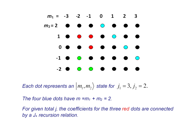
How do these dots relate to the CG coefficients? the top right-hand dot (3, 2) uniquely represents the $j = 5, m = 5$ state of total angular momentum. The next dots down, (2, 2) and

(3, 1), correspond to two CG coefficients for $j = 5$ and two different CG coefficients for $j = 4.$

If we now pick one value of $j$ less than $j_{1} + j_{2},$ each dot in the grid will correspond to one coefficient.

Note that having fixed $j,$ the grid will be curtailed: let’s take $j = 3,$ so $m = m_{1} + m_{2} = 3$ at most. Then the grid loses its far corners:

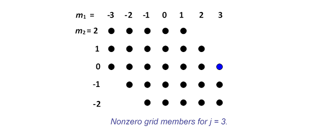
Let us examine for this fixed $j$ which CG coefficients are where in this curtailed grid.

There are a total of $2 j + 1 = 7$ states for $m = 3, 2, \dots, - 3.$

The top state, $j = 3, m = 3,$ or ${| 3, 3 〉}_{j m}$ , is given by three coefficients on the top diagonal line (it’s in a three-dimensional subspace, and orthogonal to $j = 5$ and $j = 4$ multiplet members ${| 5, 3 〉}_{j m}, {| 4, 3 〉}_{j m}$ which are also in the $m = 3$ subspace). We’re not at this point calculating these coefficients, we’re just trying to find them a home.

Applying the lowering operator to ${| 3, 3 〉}_{j m}$ gives a vector in the four-dimensional $m = 2$ subspace, the coefficients would belong to the next diagonal down, which has four elements. (This subspace also includes the top member of the $j = 2$ multiplet.) Using the lowering operator one more time we enter the five-dimensional $m = 1$ subspace $—$ but that is the maximum number of dimensions in this problem, since angular momenta 3 and 2 cannot be added to give a $j = 0$ scalar.

Having now, for this particular $j$ made from $j_{1} + j_{2}$ , found where all the CG coefficients for all the $2 j + 1$ multiplet members are located, we shall see how they can all be systematically calculated using the recursion relations generated by $J_{\pm} = J_{1 \pm} + J_{2 \pm}$ .

We’ve mapped the recursion relations on the diagram: given $j, j_{1}, j_{2}$ the three red dots at $(m_{1}, m_{2}), (m_{1} - 1, m_{2}), (m_{1}, m_{2} - 1)$ (with $m_{1} = - 1, m_{2} = 1$ in this example) locate the three CG coefficients satisfying the linear equation above from

$〈 m_{1}, m_{2} | J_{+} | j, m 〉 = 〈 m_{1}, m_{2} | J_{1 +} | j, m 〉 + 〈 m_{1}, m_{2} | J_{2 +} | j, m 〉$

so if two of them are known the third is given. Similarly, the parallel equation generated by $J_{-} = J_{1 -} + J_{2 -}$ links the three green dots, at $(m_{1}, m_{2}), (m_{1} + 1, m_{2}), (m_{1}, m_{2} + 1)$ .

We begin the computation of the CG coefficients with the blue dot, the point on the leading “arrow” edges. Let us arbitrarily assign a value 1 to this point. If we make it the top member of a “green” triangle, that will link it to the dot below and to a dot to the right which is off the array. The dot off the array makes zero contribution, so we have an equation giving the value of the coefficient at the dot below the blue dot as a multiple of the value on the blue dot. We can then continue down to the next dot. We could instead have gone up from the blue dot using incomplete red triangles $—$ in fact we can continue around the edge of the whole array. Then, once the values along the edges are fixed, the recursion triangles can be used to move inward and find the rest.

The point of this section is to establish that, apart from an overall multiplicative constant that must be fixed by normalization, all the CG coefficients for this value of $j$ can be found from the recursion relations alone. The reason this is important is because the same algebraic structure, and therefore the same recursion relations, are used to define spherical tensors, so they can also be combined using the same CG coefficients. (We still need a sign convention here to present a complete table: so far, the different values of total $j$ have arbitrary relative phases.)

previous home next PDF