Scattering Theory
Michael Fowler, UVa
References: Baym, Lectures on Quantum Mechanics, Chapter 9.
Sakurai, Modern Quantum Mechanics, Chapter 7.
Shankar, Principles of Quantum Mechanics, Chapter 19.
Introduction
Almost everything we know about nuclei and elementary
particles has been discovered in scattering experiments, from
The simplest model of a scattering experiment is given by solving Schrödinger’s equation for a plane wave impinging on a localized potential. A potential might represent what a fast electron encounters on striking an atom, or an alpha particle a nucleus. Obviously, representing any such system by a potential is only a beginning, but in certain energy ranges it is quite reasonable, and we have to start somewhere!
The basic scenario is to shoot in a stream of particles, all at the same energy, and detect how many are deflected into a battery of detectors which measure angles of deflection. We assume all the ingoing particles are represented by wavepackets of the same shape and size, so we should solve Schrödinger’s time-dependent equation for such a wave packet and find the probability amplitudes for outgoing waves in different directions at some later time after scattering has taken place. But we adopt a simpler approach: we assume the wavepacket has a well-defined energy (and hence momentum), so it is many wavelengths long. This means that during the scattering process it looks a lot like a plane wave, and for a period of time the scattering is time independent. We assume, then, that the problem is well approximated by solving the time-independent Schrödinger equation with an ingoing plane wave. This is much easier!
All we can detect are outgoing waves far outside the region of scattering. For an ingoing plane wave , the wavefunction far away from the scattering region must have the form
where are measured with respect to the ingoing direction.
Note that the scattering amplitude has the dimensions of length.
We don’t worry about overall normalization, because what is relevant is the fraction of the incoming beam scattered in a particular direction, or, to be more precise, into a small solid angle in the direction The ingoing particle current (with the above normalization) is through unit area perpendicular to the ingoing beam, the outgoing current into the small angle is . It is evident that this outgoing current corresponds to the original ingoing current flowing through a perpendicular area of size , and
is called the differential cross section for scattering in the direction
The Time-Independent Description
We shall review the time-independent formulation of scattering theory, first as it is presented in Baym, in terms of the standard Schrödinger equation wavefunctions, then do the same thing a la Sakurai, in the more formal, but of course equivalent, language of bras and kets. The Schrödinger wavefunction approach is an easier introduction, but the formal language is more convenient for analyzing the structure of higher order terms.
Actually, Baym’s treatment isn’t quite time-independent, in that he uses an ingoing wavepacket, but it is one of great length, well approximated by a plane wave. Sakurai goes straight to the plane wave, and we do too. This case is very reminiscent of one-dimensional scattering, in which a plane wave from the left generates outgoing waves in both directions, and the amplitudes can be calculated from the Schrödinger equation for a single energy eigenstate. The only difference is that in 3D there will be outgoing waves in all directions.
Following Baym, Schrödinger’s equation is:
This we take to have an incoming plane wave component . Overall normalization is irrelevant, since the differential cross-section depends only on the ratio of the scattered wave amplitude to that of the ingoing wave.
The standard approach to an equation like the one above is to transform it into an integral equation using Green’s functions. If is small (just how small it has to be will become clear later) the integral equation can then be solved by iteration.
The Green’s function is essentially the inverse of the differential operator,
This is not a mathematically unique definition: clearly, we can add to any solution of the homogeneous equation
for example, the incoming plane wave.
If we write the integral equation
this is certainly a solution to the original Schrödinger equation, as is easily checked by applying the operator
to both sides of the equation.
The integral equation can be formally solved by iteration, and for “small” the solution will converge. But this won’t really doremember, we haven’t a unique ! We have to fix by connecting better with the scattering problem we’re trying to solve.
We know our solution has a single ingoing plane wave, and outgoing waves in all other directions, generated by the interaction of the plane wave with the potential. But the Schrödinger equation could equally describe ingoing waves in the other directions. In defining the Green’s function and writing the integral equation, we have nowhere specified the distant form of the wavefunction, that is, we have not required that the Green’s function on the right hand side of the integral equation only generate outgoing waves. To see how to do this, we must write the Green’s function itself as a sum over waves, in other words a Fourier transform, and see how to eliminate the unphysical (for the present problem) incoming waves in that sum.
The explicit form of the Green’s function is
Note that only depends on through and only on through since the integration over is over all directions. It is easy to verify that this Green’s function satisfies the differential equation, by applying the differential operator to the first integral above: the result is to cancel the denominator in the integral, leaving just , which is the function in
To get the second form of in the equation above, we first do the angular integration to get , then rearrange the integral over the term by switching the sign of , so it becomes an integral from to 0 instead of 0 to Then we add the two terms (the and the ) together to give an integral from This integral from is then done by contour integrationat least, after we’ve figured out what to do about the singularities at
For the integral to be defined, the contour must be distorted slightly so it bypasses these poles.
It is at this point we feed in our physical knowledge of the situation: that in the scattering process, the second term in
that is, the Green’s function term, has to be a sum over outgoing waves only. And, we can guarantee this by distorting the contour of integration in the right direction, as follows.
The contour integral has to be evaluated by closing the contour. Since r is positive goes to zero in the upper half plane, but diverges in the lower half, so we must close the contour in the upper half plane to ensure no contribution from the semicircle at infinity. Therefore, to get the desired outgoing waves, but not our contour closed in the upper half plane must encircle the pole at but not the one at ( does represent outgoing waves: the suppressed time dependence is , giving .) In other words, the relative configuration of the real-axis part of the contour and the two poles has to be:
x (pole)
x (pole at ) (pole at )
Instead of moving the contour slightly off the real axis to avoid the poles, we’ve moved the poles slightly instead. These movements are infinitesimal, so which gets moved makes no difference to the value of the integral. It is more convenient to move the poles, as shown, because this move can be efficiently included in the integral just by adding an infinitesimal imaginary part to the denominator:
Notice that we have written instead of because can denote any solution of
and we are specifying the particular solution having only outgoing waves. In contrast to is well-defined and unique. (There is another perfectly valid solution having only ingoing waves, but it is irrelevant to the scattering problem. The difference between the ingoing and outgoing solutions satisfies the homogeneous equation having zero on the right-hand side.)
Once we move the poles slightly as described above, the pole at is in fact the only singularity of the integrand lying inside the contour of integration (closed in the upper half plane), so the value of the integral is just the contribution from this pole, that is,
.
Therefore the prescription (as it’s sometimes called) in does indeed give us what we want: a solution having only outgoing waves, and the integral equation becomes:
This can be written more simply if we assume the potential to be localized, so that we can take In this case, it is a good approximation to take in the denominator. However, this approximation cannot be made in the exponential, because to leading order (see diagram)
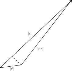
and although the second term is much smaller than the first, it is a phase, which may be of order unity. Such a factor must of course be included so that the contributions to the integral from different regions of the potential are added with the correct relative phases.
Therefore, assuming the detector distance is much larger than the range of the potential, we can write
The Born Approximation
From the above equation, the first order approximation to the scattering is given by replacing in the integral on the right with the zeroth-order term
This is the Born approximation. In terms of the scattering amplitude which we defined in terms of the asymptotic wave function:
the Born approximation is:
where is the momentum transfer, . (Since the incoming and outgoing momenta have equal magnitude, it is easy to check that )
The essential physics here is that a particle scattered with momentum change is scattered by the -Fourier component of the potentialone can imagine the potential as built up of Fourier components each of which acts like a diffraction grating. Higher order corrections to the Born approximation correspond to successive scatterings off these gratingsthese higher orders are generated by iteration of
It is important to establish when the Born approximation is a good one: sometimes it isn’t. Actually, we are just doing perturbation theory in disguise, so we need the perturbation to be small, that is to say, replacing by in the integral on the right in the equation above should only make a small difference to the value of given by doing the integral. This is of course a rather tricky exercise in self-consistency.
Let us attempt to estimate what difference the replacement of by in the integrand does make for the common case of a spherically symmetric potential parameterized by depth and range The integral is effectively only over a region of size around the origin.
First consider low energy scattering, say, so for estimation purposes we can replace the exponential term by 1 in the region of integration. We also assume that where appears in the integral on the right-hand side of the equation is also pretty close to 1 (remember the integral is only over a volume within or so of the origin) and so we just replace it by 1. In other words, we’re assuming that the ingoing plane wave, the , is not dramatically distorted inside that volume where the potential is significant.
Now, we’ve assumed the wave function near the origin is close to 1, so putting that value in the integrand on the right had better give a value for on the left hand side of the equation which is pretty close to 1. The approximations give:
so the Born approximation will be reasonable at low energies ( ) if the second term on the right hand side is a lot less than unity.
When is this true for a real potential? Taking to have depth and range the Born approximation is good if:
Notice that the right hand side of this inequality is of order the kinetic energy of a particle confined to a volume equal to the range of the potential, so the Born approximation is valid at low energies provided the potential is well below the strength necessary for a bound state.
In fact, the Born approximation works better at higher energies, because the oscillating phase term in cuts down the value of the integral by a factor of order of magnitude . This means the condition becomes always satisfied at high enough energies.
The Lippmann-Schwinger Equation
It proves illuminating, especially in understanding scattering beyond the Born approximation, to recast the Green’s function derivation of the scattering amplitude in the more formal language of bras, kets and operators. The Green’s function was introduced in the previous section as the (non-unique) inverse of the operator
.
(Parenthetical remark: in numerical computation, the wavefunction might be specified at points on a lattice in space, and a differential operator like this would be represented as a difference operator, that is, as a large but finite matrix operating on a large vector whose elements were the wavefunction values at points on the lattice. The Green’s function would then be the inverse matrix with appropriate boundary conditions specified to ensure uniqueness.)
Purely formally (and following Sakurai), writing with the kinetic energy operator , the ingoing plane wave state is a solution of
We want to solve
The transformation from a differential equation to an integral equation in this language is:
This gives the undisturbed incoming wave for and by operating on both sides of the equation with we find does indeed satisfy the full Schrödinger equation. But of course this transformation from a differential to an integral equation has the same flaw as the earlier treatment: has a continuum of eigenvalues in the infinite volume limit, so the operator equation becomes ill-defined for those eigenstates with energy arbitrarily close to the incoming energy, and those are precisely the states of physical relevance.
To make explicit that this is indeed the problem we’ve already solved, let us translate it into the earlier language. First take the inner product with the bra
Next, insert a representation of unity as a sum over eigenstates of momentum (and therefore of ) into the last term:
Finally, insert another representation of unity as a sum over eigenstates of position in the last term:
Comparing this expression with the integral equation in the earlier discussion, it is evident that they are indeed equivalent, and therefore the correct prescription to give the scattered wave function,
where
in which form it is evident that is the same as in the previous work.
This equation for the scattered wave is called the Lippmann-Schwinger equation.
Note : Sakurai defines his Green’s function as
Now that we have a well-defined Green’s function operator the Lippmann-Schwinger equation can be solved formally:
with a series solution
just a formal version of the solution we found earlier.
The Transition Matrix
Operating on both sides of the above the equation with
defining the “transition matrix” by
In terms of this transition matrix operator, the scattered wave can be written
Comparing this with
,
and recalling that the Born approximation is given by
,
we see that is a kind of generalized potential, including all the higher order terms, so that just as the Born approximation gave the scattering amplitude in terms of
the exact result including all higher order terms must have the same structure with replacing Of course, unlike is not a diagonal matrix in space: it depends on two space variables, and its Fourier transform is a therefore function of two momenta, that is, the incoming and the scattered . Thus we find:
We have replaced the in the Born expression with . Sakurai has an extra in the term on the right, because he uses , , we use , .
The Optical Theorem
The Optical Theorem relates the imaginary part of the forward scattering amplitude to the total cross-section,
The physical content of this initially mysterious theorem will become a lot clearer after we discuss partial waves and some geometric effects. It does tell us that cannot be real in all directions, and that in particular has a positive imaginary part in the forward direction. We’ve included the proof here for the record, but you can skip it for now. But note that this proof is more general than the simple one given (later) in the section on partial waves, in that we do not here assume the potential to have spherical symmetry.
From the expression for above, we see that we must find the imaginary part of
Recall that
so we need to find
Since is hermitian, the only imaginary part of the above matrix element comes from the recalling that
Therefore,
Again using
we can rewrite the equation
Inserting a complete set of plane wave states in the final matrix element above gives
(This is the same formula as Sakurai’s in 7.3: our extra in the denominator is only apparent, because our plane wave states differ from his by a factor )
Time-Dependent Formulation of Scattering Theory
In the time-independent formulation presented above, we solved the Lippmann-Schwinger equation to find
where
and
(Reminder on our wave function normalization convention: we always have a denominator for an integral This means the identity operator as a sum over plane wave projection operators is . The normalization is , and . Sakurai uses , and as does Shankar in Chapter 1, for one dimension, page 67, but later, Chapter 21 page 585, Shankar has switched to our notationso watch out! Our convention is also used by Baym and by Peskin.)
In fact, this function is the Fourier transform of the propagator we discussed last semester. To see how this comes about, take the matrix element between two position eigenstates and Fourier transform from energy to time:
The integral over is along the real axis, and the contour is closed in the half plane where the integrand goes to zero for in the imaginary direction, that is, in the lower half plane for and the upper half plane for But with the term shown, all the singularities of the integrand are in the lower half plane. Hence is identically zero for
For is just the free particle propagator between the two points (apart from the phase factor ):
To summarize: terms in the series solution of the Lippmann-Schwinger equation can be interpreted as successive scatterings off the Fourier components of a potential, with plane wave propagation in between, with the sign of the term ensuring that there are only outgoing waves from each scattering. In the Fourier transformed version above, the sum is over scattering at all possible points where the potential is nonzero, with propagation in between, the ensuring that the scattering path only moves forward in time.
Last semester, we defined the free-particle propagator as the operator The propagator describes development of the free-particle wave function in time, so naturally Then Fourier transforming the propagator from to and inserting an infinitesimal exponentially decaying factor to define the integral at infinity, we find
Note that the propagators and differ by a factor of specifically
We follow Sakurai’s (section 7.11) notation, this is the correctly normalized Green’s function for the time-dependent free-particle Schrödinger equation: it is the solution of
which propagates forwards in time. The reason the propagators and differ by a factor of is that the Lippmann-Schwinger equation can be generated as a time sequence using the higher-order perturbation theory interaction representation described earlier in the course, essentially expanding as a time-ordered series expansion in and each factor has an accompanying these factors are taken care of by using instead of
Exercise: in that earlier lecture, we gave the second-order term as:
Assume that the potential is constant in time. Fourier transform this expression from to and establish that it has the structure .
The Born Cross-Section from Time-Dependent Theory
We established in the lecture on Time-Dependent Perturbation Theory that to leading order in the perturbation, the transition rate from an initial state to a final state is given by Fermi’s Golden Rule:
We can use this result to findin leading orderthe rate of scattering from an incoming plane wave into any outgoing plane wave state having the same energy, and hence by adding the rate over the plane wave directions pointing within a given small solid angle rederive the Born approximation.
Conceptually, though, this is a bit tricky. From the above solution of the Schrödinger equation, we know the outgoing wave is a spherical one, so in a particular direction the amplitude decreases. But that doesn’t happen with a plane wave! The clearest way to handle this is to put the system in a big box, a cube of side with periodic boundary conditions. This makes it easier to count states and normalize the plane waves properlyof course, in the limit of a large box, the plane waves form a complete set, so any spherical wave can be expressed as a sum over these plane waves.
In this section, then, we use box-normalized plane waves:
So
where the momentum transfer to the particle
It is important to note that we are taking the incoming wave to be just one of the normalized plane wave states satisfying the box periodic boundary conditions, so now the incoming current, being from just one of these plane waves, is
The Golden Rule becomes
denoting a plane wave going outwards within the solid angle
Now, the function simply counts the number of states available at the correct (initial) energy, within the specified final solid angle of direction. The density of states in momentum space (for volume of real space) is one state in each momentum-space volume so using the density of states in energy for outgoing solid angle is .
Putting this all together
The transition rate, the rate of scattering into is just the incident current multiplied by the infinitesimal scattering cross-section (that was our definition of ),
because our definition of included the appropriately normalized ingoing wave.
so finally
Footnote: the continuum version.
In the continuum version, , so the matrix element term is just The energy function is only meaningful inside an integral, in this case over the small volume of outgoing scattering states in the solid angle and energy equal to the ingoing energy. But this integral over space must include the factor, according to our rule, giving an outgoing phase space term
This establishes that our continuum normalization conventions give the same result as that obtained from box normalization.
Electrons Scattering from Atoms
This same approach, using the Golden Rule to derive the leading order scattering rate, is useful is analyzing the scattering of fast electrons by atoms. The problem with slow electrons is that the wave function needs to be antisymmetric with respect to all electrons present. We assume fast electrons have little overlap with the atomic electron wave functions in momentum space, so we don’t have to worry about symmetry.
With this approximation, following Sakurai (page 431) the scattering amplitude matrix element is
where the potential term is that from the nucleus, plus the repulsion from the other electrons at positions Taking the final atomic state allows for the possibility of inelastic scattering.
Since the distance of the scattered electron from the nucleus has nothing to do with the atomic state, for the nuclear contribution, which is then just Coulomb scattering, and
(To do this integral, put in a convergence factor then let )
The term involving the atomic electrons is another matter: for the electron, integrating over the coordinate of the scattered electron gives a factor , but the hard part is finding the value of the matrix element of this operator between the atomic states. Notice that this is just the Fourier transform of the electrostatic potential from the electron’s charge density,
transforms to and Fourier transforms to .
The Form Factor
For elastic scattering, then, the contribution of the atomic electrons is simply interpreted: their charge density gives rise to a potential by the usual electrostatic equation, and the (fast) electron is scattered by this potential. For inelastic scattering, the Fourier transform of the electron density is evaluated between different atomic states. In both cases, the matrix element is called the form factor for the scattering, actually The normalizing factor is introduced so that for elastic scattering, as .
So the form factor is a map of the charge density in space. By measuring the scattering rate at different angles, and Fourier analyzing, it is possible to delineate the charge distribution in ordinary space. The same technique works for nuclei, and in fact for particlesthe neutron, for example, although electrically neutral, has a nontrivial electrical charge distribution within its volume, revealed by scattering very fast electrons.
More general form factors describe distribution of spin, and also time dependence of distributions of charge or spin in excited systems. These can all be measured with suitably designed scattering experiments.