More Scattering: the Partial Wave Expansion
Michael Fowler, UVa
Plane Waves and Partial Waves
We are considering the solution to Schrödinger’s equation for scattering of an incoming plane wave in the z-direction by a potential localized in a region near the origin, so that the total wave function beyond the range of the potential has the form
The overall normalization is of no concern, we are only interested in the fraction of the ingoing wave that is scattered. Clearly the outgoing current generated by scattering into a solid angle at angle is multiplied by a velocity factor that also appears in the incoming wave.
Many potentials in nature are spherically symmetric, or nearly so, and from a theorist’s point of view it would be nice if the experimentalists could exploit this symmetry by arranging to send in spherical waves corresponding to different angular momenta rather than breaking the symmetry by choosing a particular direction. Unfortunately, this is difficult to arrange, and we must be satisfied with the remaining azimuthal symmetry of rotations about the ingoing beam direction.
In fact, though, a full analysis of the outgoing scattered waves from an ingoing plane wave yields the same information as would spherical wave scattering. This is because a plane wave can actually be written as a sum over spherical waves:
Visualizing this plane wave flowing past the origin, it is clear that in spherical terms the plane wave contains both incoming and outgoing spherical waves. As we shall discuss in more detail in the next few pages, the real function is a standing wave, made up of incoming and outgoing waves of equal amplitude.
We are, obviously, interested only in the outgoing spherical waves that originate by scattering from the potential, so we must be careful not to confuse the pre-existing outgoing wave components of the plane wave with the new outgoing waves generated by the potential.
The radial functions appearing in the above expansion of a plane wave in its spherical components are the spherical Bessel functions, discussed below. The azimuthal rotational symmetry of plane wave + spherical potential around the direction of the ingoing wave ensures that the angular dependence of the wave function is just , not . The coefficient is derived in Landau and Lifshitz, §34, by comparing the coefficient of on the two sides of the equation: as we shall see below, does not appear in for greater than and does not appear in for less than so the combination only occurs oncein the term, and the coefficients on both sides of the equation can be matched. (To get the coefficient right, we must of course specify the normalizations for the Bessel functionsee belowand the Legendre polynomial.)
Mathematical Interval: The Spherical Bessel and Neumann Functions
The plane wave is a trivial solution of Schrödinger’s equation with zero potential, and therefore, since the form a linearly independent set, each term in the plane wave series must be itself a solution to the zero-potential Schrödinger’s equation. It follows that satisfies the zero-potential radial Schrödinger equation:
The standard substitution yields
For the simple case the two solutions are . The corresponding radial functions are (apart from overall constants) the zeroth-order Bessel and Neumann functions respectively.
The standard normalization for the zeroth-order Bessel function is
and the zeroth-order Neumann function
Note that the Bessel function is the one well-behaved at the origin: it could be generated by integrating out from the origin with initial boundary conditions of value one, slope zero.
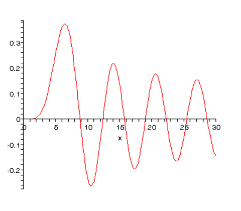
Here is a plot of from

For nonzero near the origin The well-behaved solution is the Bessel function, the singular function the Neumann function. The standard normalizations of these functions are given below.
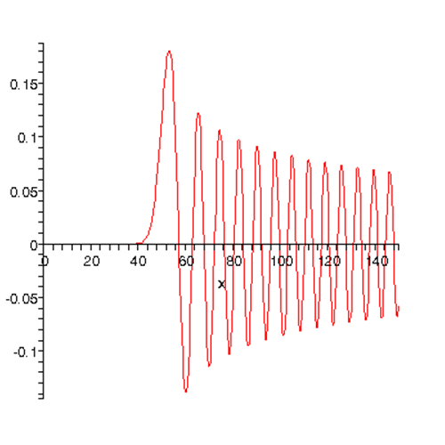
Here are :
Detailed Derivation of Bessel and Neumann Functions
This subsection is just here for completeness. We use the dimensionless variable
To find the higher solutions, we follow a clever trick given in Landau and Lifshitz (§33).
Factor out the behavior near the origin by writing
The function satisfies
The trick is to differentiate this equation with respect to
Writing purely formally , the equation becomes
But this is the equation that must obey! So we have a recursion formula for generating all the from the zeroth one: and , up to a normalization constant fixed by convention.
In fact, the standard normalization is
Now
This is a sum of only even powers of It is easily checked that operating on this series with can never generate any negative powers of It follows that written as a power series in has leading term proportional to The coefficient of this leading term can be found by applying the differential operator to the series for
This behavior near the origin is the usual well-behaved solution to Schrödinger’s equation in the region where the centrifugal term dominates.
Note that the small behavior is not immediately evident from the usual presentation of the ’s, written as a mix of powers and trigonometric functions, for example
Turning now to the behavior of the ’s for large from
it is evident that the dominant term in the large regime (the one of order ) is generated by differentiating only the trigonometric function at each step. Each such differentiation can be seen to be equivalent to multiplying by (-1) and subtracting from the argument, so
These then, are the physical partial-wave solutions to the Schrödinger equation with zero potential. When a potential is turned on, the wave function near the origin is still (assuming, as we always do, that the potential is negligible compared with the term sufficiently close to the origin). The wave function beyond the range of the potential can be found numerically in principle by integrating out from the origin, and in fact will be like above except that there will be an extra phase factor, called the “phase shift” and denoted by ) in the sine. The significance of this is that in the far region, the wave function is a linear combination of the Bessel function and the Neumann function (the solution to the zero-potential Schrödinger equation singular at the origin). It is therefore necessary to review the Neumann functions as well.
As stated above, the Neumann function is
the minus sign being the standard convention.
An argument parallel to the one above for the Bessel functions establishes that the higher-order Neumann functions are given by:
Near the origin
and for large
so a function of the form asymptotically can be written as a linear combination of Bessel and Neumann functions in that region.
Finally, the spherical Hankel functions are just the combinations of Bessel and Neumann functions that look like outgoing or incoming plane waves in the asymptotic region:
so for large
The Partial Wave Scattering Matrix
Let us imagine for a moment that we could just send in a (time-independent) spherical wave, with variation given by For this partial wave (dropping overall normalization constants as usual) the radial function far from the origin for zero potential is
If now the (spherically symmetric) potential is turned on, the only possible change to this standing wave solution in the faraway region (where the potential is zero) is a phase shift
This is what we would find on integrating the Schrödinger equation out from nonsingular behavior at the origin.
But in practice, the ingoing wave is given, and its phase cannot be affected by switching on the potential. Yet we must still have the solution to the same Schrödinger equation, so to match with the result above we multiply the whole partial wave function by the phase factor . The result is to put twice the phase change onto the outgoing wave, so that when the potential is switched on the change in the asymptotic wave function must be
This equation introduces the scattering matrix
which must lie on the unit circle to conserve probabilitythe outgoing current must equal the ingoing current. If there is no scattering, that is, zero phase shift, the scattering matrix is unity.
It should be noted that when the radial Schrödinger’s equation is solved for a nonzero potential by integrating out from the origin, with initially, the real function thus generated differs from the wave function given above by an overall phase factor .
Scattering of a Plane Wave
We’re now ready to take the ingoing plane wave, break it into its partial wave components corresponding to different angular momenta, have the partial waves individually phase shifted by dependent phases, and add it all back together to get the original plane wave plus the scattered wave.
We are only interested here in the wave function far away from the potential. In this region, the original plane wave is
Switching on the potential phase shifts factor the outgoing wave:
The actual scattering by the potential is the difference between these two terms. The complete wave function in the far region (including the incoming plane wave) is therefore:
The factor cancelled the The -1 in is there because zero scattering means Alternatively, it could be regarded as subtracting off the outgoing waves already present in the plane wave, as discussed above. There is no dependence since with the potential being spherically-symmetric the whole problem is azimuthally-symmetric about the direction of the incoming wave.
It is perhaps worth mentioning that for scattering in just one partial wave, the outgoing current is equal to the ingoing current, whether there is a phase shift or not. So, if switching on the potential does not affect the total current scattered in any partial wave, how can it cause any scattering? The point is that for an ingoing plane wave with zero potential, the ingoing and outgoing components have the right relative phase to add to a component of a plane wavea tautology, perhaps. But if an extra phase is introduced into the outgoing wave only, the ingoing + outgoing will no longer give a plane wavethere will be an extra outgoing part proportional to .
Recall that the scattering amplitude was defined in terms of the solution to Schrödinger’s equation having an ingoing plane wave by
We’re now ready to express the scattering amplitude in terms of the partial wave phase shifts (for a spherically symmetric potential, of course):
where
is called the partial wave scattering amplitude, or just the partial wave amplitude.
So the total scattering amplitude is the sum of these partial wave amplitudes:
The total scattering cross-section
gives
So the total cross-section is the sum of the cross-sections for each value. This does not mean, though, that the differential cross-section for scattering into a given solid angle is a sum over separate valuesthe different components interfere. It is only when all angles are integrated over that the orthogonality of the Legendre polynomials guarantees that the cross-terms vanish.
Notice that the maximum possible scattering cross-section for particles in angular momentum state is which is four times the classical cross section for that partial wave impinging on, say, a hard sphere! (Imagine semiclassically particles in an annular area: angular momentum say, but and so Therefore the annular area corresponding to angular momentum “between” and has inner and outer radii and and therefore area ) The quantum result is essentially a diffractive effect, we’ll discuss it more later.
It’s easy to prove the optical theorem for a spherically-symmetric potential: just take the imaginary part of each side of the equation
at using
from which the optical theorem follows immediately.
It’s also worth noting what the unitarity of the partial wave scattering matrix implies for the partial wave amplitude . Since it follows that
From this, gives:
This can be put more simply:
In fact,
Phase Shifts and Potentials: Some Examples
We assume in this section that the potential can be taken to be zero beyond some boundary radius This is an adequate approximation for all potentials found in practice except the Coulomb potential, which will be discussed separately later.
Asymptotically, then,
This expression is only exact in the limit but since the potential can be taken zero beyond the wave function must have the form
for
(The - sign comes from the standard convention for Bessel and Neumann functionssee earlier.)
The Hard Sphere
The simplest example of a scattering potential:
The wave function must equal zero at so from the above form of
For
so This amounts to the wave function being effectively moved over to begin at instead of at the origin:
for of course for
For higher angular momentum states at low energies ( ),
Therefore at low enough energy, only scattering is importantas is obvious, since an incoming particle with momentum and angular momentum is most likely at a distance from the center of the potential at closest approach, so if this is much greater than the phase shift will be small.
The Born Approximation for Partial Waves
From the definition of
and
recall the Born approximation amounts to replacing the wave function in the integral on the right by the incoming plane wave, therefore ignoring rescattering.
To translate this into a partial wave approximation, we first take the incoming to be in the direction, so in the integrand we replace by
Labeling the angle between and by
Now is in the direction and in the direction , and is the angle between them. For this situation, there is an addition theorem for spherical harmonics:
On inserting this expression and integrating over the nonzero terms give zero, in fact the only nonzero term is that with the same as the term in the expansion, giving
and remembering
it follows that for small phase shifts (the only place it’s valid) the partial-wave Born approximation reads
Low Energy Scattering: the Scattering Length
From
the cross section is
At energy the radial Schrödinger equation for away from the potential becomes , with a straight line solution This must be the limit of , which can only be correct if is itself linear in for sufficiently small and then it must be being the point at which the extrapolated external wavefunction intersects the axis (maybe at negative !) So, as goes to zero, the cot term dominates in the denominator and
The quantity is called the scattering length.
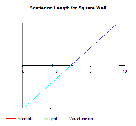
Integrating the zero-energy radial Schrödinger equation out from at the origin for a weak (spherical) square well potential, it is easy to check that is positive for a repulsive potential, negative for an attractive potential.
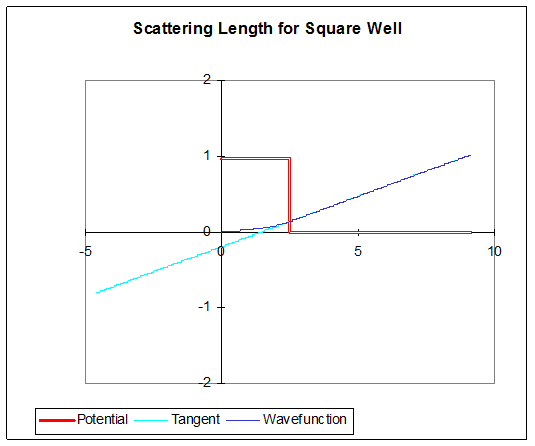
Repulsive potential, zero-energy wave function (so it’s a straight line outside of the well!):
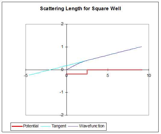
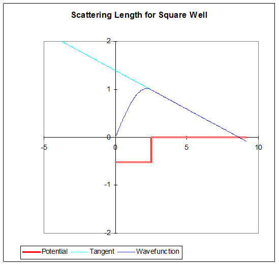
Attractive potential:
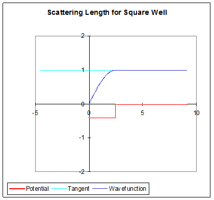
On increasing the strength of the repulsive potential, still solving for the zero-energy wave function, tends to the potential wallhere’s the zero-energy wavefunction for a barrier of height 6:
For an infinitely high barrier, the wave function is pushed out of the barrier completely, and the hard sphere result is recovered: scattering length cross-section
On increasing the strength of the attractive well, if there is a phase change greater that within the well, will become positive. In fact, right at is infinite!
And a little more depth to the well gives a positive scattering length:
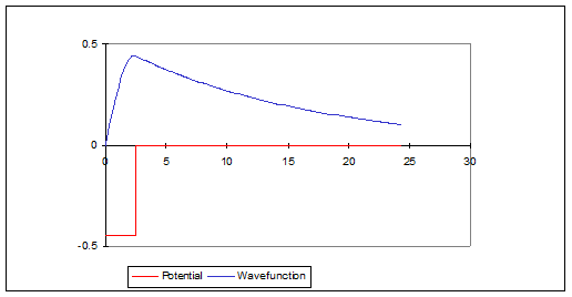
In fact, a well deep enough to have a positive scattering length will also have a bound state. This becomes evident when one considers that the depth at which the scattering length becomes infinite can be thought of as formally having a zero energy bound state, in that although the wave function outside is not normalizable, it is equivalent to an exponentially decaying function with infinite decay length. If one now deepens the well a little, the zero-energy wave function inside the well curves a little more rapidly, so the slope of the wave function at the edge of the well becomes negative, as in the picture above. With this slightly deeper well, we can now lower the energy slightly to negative values. This will have little effect on the wave function inside the well, but make possible a fit at the well edge to an exponential decay outsidea genuine bound state, with wave function outside the well.
If the binding energy of the state is really low, the zero-energy scattering wave function inside the well is almost identical to that of this very low energy bound state, and in particular the logarithmic derivative at the wall will be very close, so taking to be much larger than the radius of the well.
This connects the large scattering length to the energy of the weakly bound state,
(Sakurai, p 414.)
Wigner was the first to use this to estimate the binding energy of the deuteron from the observed cross section for low energy neutron-proton scattering.