Relating Scattering Amplitudes to Bound States
Michael Fowler, UVa.
Low Energy Approximations for the S Matrix
In this section, we examine the properties of the partial-wave scattering matrix
for complex values of the momentum variable Of course, general complex values of do not correspond to physical scattering, but it turns out that the scattering of physical waves can often be most simply understood in terms of dominant singularities in the complex plane.
We begin with the complex connection between (positive energy) scattering and (negative energy) bound states. The asymptotic form of the partial wave function in a scattering experiment is (from the previous lecture)
An bound state has asymptotic wave function
where is a normalization constant.
Notice that this resembles an “outgoing wave” with imaginary momentum If we analytically continue the scattering wave function from real into the complex plane, we get both exponentially increasing and decreasing wave functions, making no physical sense. But there is an exception to this general observation: if the scattering matrix becomes infinite at some complex value of the exponentially decreasing term will be infinitely larger than the exponentially increasing term. In other words, we’ll only have a decreasing wave functiona bound state. We know that the energy of a bound state has to be real and negative, and is also equal to so this can only happen for pure imaginary,
Now, the existence of a low energy bound state means that the matrix has a pole (on the imaginary axis) close to the origin, so this will strongly affect low energy (near the origin, but real ) scattering. Let’s see how that works using the low-energy approximation discussed previously. Recall that the partial wave amplitude
and at low energy so
and
Note that as as it should, since and . Note also that this approximation correctly gives .
This has a pole in the complex plane at and if this corresponds to a bound state having then the binding energy In fact, though, we run into a problem here: we get the same form of at low energies even for a repulsive potential, which certainly doesn’t have a bound state! The pole in only means that we can have an asymptotic wave function of the right form, but it does not guarantee that this asymptotic form will go smoothly to nonsingular behavior at the origin. For a repulsive potential, it’s easy to see that the zero (or negative) energy wave function on integrating out from the origin slopes more and more steeply upwards, so could never, with increasing go over to asymptotic decay.
Effective Range
The low energy approximation above can be written
.
We shall now derive a better approximation,
,
where called the “effective range”, gives some measure of the extent of the potential (in contrast to which, as we have seen can be arbitrarily large, even for a short-range potential).
A useful mathematical tool needed at this point is the Wronskian. For two functions the Wronskian is defined as
,
the prime denoting differentiation as usual. From this, and if satisfy the same second-order differential equation (like the Schrödinger equation with the same energy) then is constant, independent of
For the radial Schrödinger equation, asymptotically
where we now show explicitly. This asymptotic function satisfies the Schrödinger equation for zero potential, but does not have the correct physical boundary behavior at
Since in the low-energy limit the asymptotic wave function
(taking ).
From the Schrödinger equation
it is easy to check that the Wronskian of with the corresponding zero energy function satisfies:
(The term involving the potential has canceled out: is nonzero here because these two functions don’t satisfy the same differential equation, the energy terms are different.)
The corresponding functions satisfy the same Wronskian equation:
We can find a formula for the effective range by integrating the difference between these two equations from to infinity: the two solutions differ only within the range of the potential, and appropriately normalizing them, then taking the difference, gives a measure of this range.
So
For large, , so there is zero contribution from the upper end. For the properly-behaved functions go to zero, the functions are
from which, with
.
it follows immediately that
and therefore
with a low-energy limit
where
.
Now, by definition coincide outside the range of the potential, but moving from that region towards the origin, they part company when the potential kicks in, with as Therefore the integral above is a rough measure of the actual range of the potential about half of it (hence the factor of 2 in defining ). Note again the contrast with which can be infinite for a short range potential.
Coulomb Scattering and the Hydrogen Atom Bound States
One particular set of bound states in a potential we’ve spent a good deal of time on are the states of the hydrogen atom, and it is interesting to see how they relate to scattering. Recall that the asymptotic form of the bound state wave function is:
But this doesn’t have the bound-state form we found above from the analytic continuation argument, there’s an extra ! What’s going on? The problem is that in all our previous work, we assumed that if we looked far enough away from the center of the potential, the radial Schrödinger equation could be taken to be that for zero potential, to any desired accuracy. The Coulomb potential, though, does not decay fast enough with distance for this to be true. For instance, it has bound states having arbitrarily large radii.
Writing
we have
Note that the extra term in the exponent keeps on growing, without limit! We are never free of the potential.
But how does this analysis of hydrogen atom wave functions relate to positive-energy scattering states? We can just analytically continue this result back to real to find out. Replacing by gives:
So we have scattering states that are not of the standard form eitherthe phase shift is infinite, and not well-defined. But we found this result be analytically continuing from the hydrogen atom bound states. Let’s check it: let us look at the radial Schrödinger equation for positive energies at large Writing as usual, let us also put for large and we can also ignore the centrifugal barrier term, so
The equation for is
and since is slowly varying, the second derivative can be ignored, so
This leads immediately to the same form we found by analytic continuation.
Resonances and Associated Zeros
Recall in the first semester we discussed decay: an particle in a heavy nucleus can be thought of as trapped in a potential well generated by the attractive nuclear forces. A spherical square well is a workable approximation, except that this square well is at the top of a hilloutside the nucleus, the repulsive electrostatic potential is sloping down from the well edge to zero as This means that for a radioactive nucleus, although the energy level would be at negative energy for the square well on level ground, actually it’s above the bottom of the electrostatic hill, and the wave function will not be decaying but oscillating. This asymptotic wave is of course very tiny, since typically the chances of detecting the α well outside the nucleus, that is, of decay, is one in millions of years.
Now consider the reverse process: imagine we bombard a decayed nucleus with particles. If we sent in one at exactly the right energy (very difficultthis is a thought experiment!) the wave function would be exactly the same as that for decay. The wave function inside the nucleus would be huge compared with that outside, we’d never see our again. Less dramatically, if we sent in one close to that energy, the wave function would still be very large inside the nucleus, meaning that the particle would spend a long time inside before coming out again. (Recall for a particle in a roller coaster potential in one dimension, the wave function is large where the particle spends a lot of timethat’s where you’re most likely to find it.) This is a resonance: at just the right energy, the amplitude of the wave function within the potential becomes very large, analogous to the amplitude of a classical driven oscillator as the driving frequency is adjusted to the natural oscillator frequency.
Can we understand this in terms of poles in the matrix? Considered as a function of energy, the matrix has poles at negative energies corresponding to bound states. But this is a positive energyand for positive energies: that’s the regime of real physical scattering. What it can have is a pole near a positive energy, in the complex plane. To keep , it would then have to have a zero at the mirror image point, that is, be locally of the form
From this,
,
so
,
and the scattering cross section reaches its maximum possible value, recall
,
so
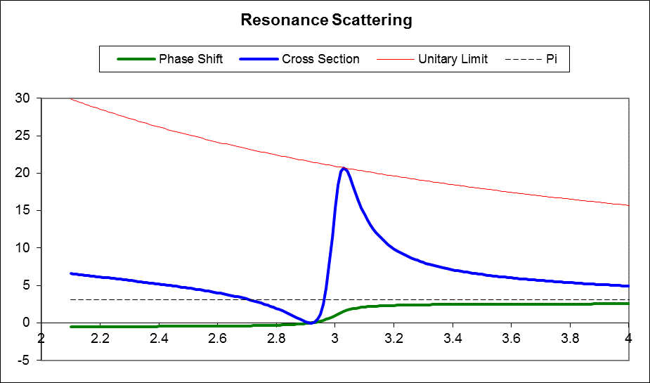
For a narrow resonance (small ) the phase shift goes rapidly from 0 to as the energy is increased through Most of the variation occurs within an energy range of is called the width of the resonance. If the resonance is superimposed on a slowly varying background phase shift then it causes an increase from to This will pass through 0 or depending on the initial sign of so the maximum scattering at phase shift will have associated with it an energy at which there is zero scattering. For substantial background the zero could be close to the peak, as illustrated below: