Oscillations III: Damped Driven Oscillator

Michael Fowler

A Driven Damped Oscillator: Equation of Motion

Here we take the damped oscillator analyzed in the previous lecture and add a periodic external driving force. If this driving force has the same period as the oscillator, the amplitude can increase, perhaps to disastrous proportions, as in the famous case of the Tacoma Narrows Bridge.

The equation of motion for a driven damped oscillator is:

_{$m \frac{d^{2} x}{d t^{2}} + b \frac{d x}{d t} + k x = F_{0} \cos ω t .$}

We shall be using $ω$ for the driving frequency, and $ω_{0}$ for the natural frequency of the oscillator (meaning that ignoring damping, so $ω_{0} = \sqrt{k / m} .$ )

The Driven Steady State Solution and Initial Transient Behavior

To get a general idea of how a damped driven oscillator behaves under a wide variety of conditions, start by exploring with our applet.

(Another approach we have used is a spreadsheet—it gives instant precise results, and can be animated, but is perhaps less intuitive.)

The solution to the differential equation above is not unique: as with any second order differential equation, there are two constants of integration, which are determined by specifying the initial position and velocity.

However, as we shall prove below using complex numbers, the equation does have a unique steady state solution with $x$ oscillating at the same frequency as the external drive. How can that be fitted to arbitrary initial conditions? The key is that we can add to the steady state solution any solution of the undriven equation $m \frac{d^{2} x}{d t^{2}} + b \frac{d x}{d t} + k x = 0,$ and we’ll clearly still have a solution of the full damped driven equation.

We know what those undriven solutions look like: they all die away as time goes on. So, we can add such a solution to fit the specified initial conditions, and after a while the system will lose memory of those conditions and settle into the steady driven solution. The initial deviations from the steady solution needed to satisfy initial conditions are termed transients.

Here’s a pair of examples: the same driven damped oscillator, started with zero velocity, once from the origin and once from 0.5:

Notice that after about 70 seconds, the two curves are the same, both in amplitude and phase.

A much clearer illustration is the initial conditions applet: two quite different complicated curves are drawn in real time, then a click reveals that the difference between the two behaves very smoothly. Try it—then put in different initial conditions.

Using Complex Numbers to Solve the Driven Steady State Equation Easily

We begin by writing:

external driving force = $F_{0} e^{i ω t}$

with $F_{0}$ real, so the actual physical driving force is just the real part of this, that is, $F_{0} \cos ω t .$

So now we’re trying to solve the equation

$m \frac{d^{2} x}{d t^{2}} + b \frac{d x}{d t} + k x = F_{0} e^{i ω t} .$

We’ll try the complex function, $x (t) = A e^{i (ω t + φ)}$ , with $A$ a real number, $x (t)$ cycling at the same frequency as the driving force. We can always take the amplitude $A$ to be real: that is not a restriction, since we’ve added the adjustable phase factor $e^{i φ} .$ Physically, this factor allows the solution to differ from the driver in phase, which it usually does. If we succeed in finding an $x (t)$ that satisfies the equation, the real parts of the two sides of the equation must be equal:

If $x (t) = A e^{i (ω t + φ)}$ is a solution to the equation with the complex driving force, $F_{0} e^{i ω t},$ its real part, $A \cos (ω t + φ),$ will be a solution to the equation with the real physical driving force, $F_{0} \cos ω t$ .

It’s very easy to check that $x (t) = A e^{i (ω t + φ)}$ is a solution to the equation, with the right $A$ and $φ$ ! Just plug it in and see what happens. The differentiations are simple, giving

$- m ω^{2} A e^{i (ω t + φ)} + i b ω A e^{i (ω t + φ)} + k A e^{i (ω t + φ)} = F_{0} e^{i ω t} .$

To nail down $A$ and $φ,$ we begin by cancelling out the common factor $e^{i ω t},$ then shift the $e^{i φ}$ to the other side to find

$A = \frac{F_{0} e^{- i φ}}{k - m ω^{2} + i b ω} .$

Now $A$ is a real number, and the right hand side of this equation looks alarmingly complex, so what’s going on?

Let’s begin to untangle this by diagramming that complex number in the denominator,

$k - m ω^{2} + i b ω$ .

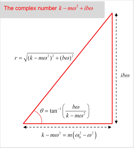
It has real part $k - m ω^{2}$ and imaginary part $i b ω .$ .

Like any complex number, it can be expressed in terms of its amplitude $r$ and its phase $θ :$

$k - m ω^{2} + i b ω = r e^{i θ}$ .

Putting it in the equation in this $r, θ$ notation gives

$A = \frac{F_{0} e^{- i φ}}{k - m ω^{2} + i b ω} = \frac{F_{0} e^{- i φ}}{r e^{i θ}} = \frac{F_{0}}{r} e^{- i (φ + θ)} .$

Now, $F_{0}$ and $r$ are real, so $A$ will be real (as it must be) if $e^{- i (φ + θ)}$ is real: so $φ = - θ,$ and

$A = \frac{F_{0}}{r} = \frac{F_{0}}{\sqrt{m^{2} {(ω_{0}^{2} - ω^{2})}^{2} + {(b ω)}^{2}}}, x (t) = A e^{i (ω t - θ)},$

recalling $k = m ω_{0}^{2}$ , and here $θ = \tan^{- 1} (\frac{b ω}{k - m ω^{2}})$ (see diagram).

So we’ve already solved the differential equation: the amplitude $A$ is proportional to the strength of the driving force, and that ratio is determined by the parameters of the undriven oscillator, and the driving oscillation frequency.

The important thing to note about the amplitude $A$ is that if the damping $b$ is small, $A$ gets very large when the frequency of the driver approaches the natural frequency of the oscillator! This is called resonance, and is what happened to the Tacoma Narrows Bridge. Of course, it has its positive aspects, from getting a swing going to tuning a radio.

The phase lag of the oscillations behind the driver, $θ = \tan^{- 1} (b ω / (k - m ω^{2}))$ , is completely determined by the frequency together with the physical constants of the undriven oscillator: the mass, spring constant, and damping strength. So, when the driving force $F_{0} e^{i ω t}$ generates the motion $x (t) = A e^{i (ω t + φ)} = A e^{i (ω t - θ)}$ , the lag angle $θ$ is independent of the strength of the driving force: a stronger force doesn’t get the oscillator more in sync, it just increases the amplitude of the oscillations.

Note that at low frequencies, $ω ≪ ω_{0},$ the oscillator lags behind by a small angle, but at resonance $ω = ω_{0} θ = π / 2,$ and for driving frequencies above $ω_{0},$ $θ > π / 2.$

Back to Reality

To summarize: we’ve just established that $x (t) = A e^{i (ω t - θ)}$ with $A = F_{0} / \sqrt{m^{2} {(ω_{0}^{2} - ω^{2})}^{2} + {(b ω)}^{2}}$ and $θ = \tan^{- 1} (b ω / (k - m ω^{2}))$ is a solution to the driven damped oscillator equation $m \frac{d^{2} x}{d t^{2}} + b \frac{d x}{d t} + k x = F_{0} e^{i ω t}$ with the complex driving force $F_{0} e^{i ω t} .$

So, equating the real parts of the two sides of the equation, since $m, b, k$ are all real,

$x = A \cos (ω t - θ)$

is a solution of the equation with the real driving force $F_{0} \cos ω t$ .

We could have found this out without complex numbers, by using a trial solution $A \cos (ω t + φ) .$ However, it’s not that easy $—$ the left hand side becomes a mix of sines and cosines, and one needs to use trig identities to sort it all out. With a little practice, the complex method is easier and is certainly more direct.

Now the total energy of the oscillator is

$\begin{matrix} E = \frac{1}{2} m v^{2} + \frac{1}{2} k x^{2} \\ = \frac{1}{2} m v^{2} + \frac{1}{2} m ω_{0}^{2} x^{2} . \end{matrix}$

Putting in

$x (t) = A \cos (ω t - θ), v (t) = - A ω \sin (ω t - θ)$

gives

$E = \frac{1}{2} m A^{2} (ω^{2} \sin^{2} (ω t - θ) + ω_{0}^{2} \cos^{2} (ω t - θ)) .$

Note that this is not constant through the cycle unless the oscillator is at resonance, $ω = ω_{0} .$

We can see from the above that at the resonant frequency $ω = ω_{0},$ $E = \frac{1}{2} m ω_{0}^{2} A^{2}$ , and from the previous section

$A = \frac{F_{0}}{\sqrt{m^{2} {(ω_{0}^{2} - ω^{2})}^{2} + {(b ω)}^{2}}},$

so the energy in the oscillator at the resonant frequency is

$E_{resonance} = \frac{1}{2} m ω_{0}^{2} A^{2} = \frac{1}{2} m ω_{0}^{2} \frac{F_{0}^{2}}{b^{2} ω_{0}^{2}} = \frac{1}{2} m \frac{F_{0}^{2}}{b^{2}} = \frac{Q^{2}}{2} \frac{F_{0}^{2}}{m ω_{0}^{2}},$

recalling that $Q = ω_{0} τ = ω_{0} m / b .$

So Q, the quality factor, the measure of how long an oscillator keeps ringing, also measures the strength of response of the oscillator to an external driver at the resonant frequency.

But what happens on going away from the resonant frequency? Let’s assume that $Q$ is large, and the driving force is kept constant. It won’t take much change in $ω$ from $ω_{0}$ for the denominator $m^{2} {(ω_{0}^{2} - ω^{2})}^{2} + {(b ω)}^{2}$ in the expression for $E$ to double in size. In fact, for large $Q$ it’s a good approximation to replace $b ω$ by $b ω_{0}$ over that variation, and it is then straightforward to check that the energy in the oscillator drops to one-half its resonant value for $ω - ω_{0} ≅ \pm ω_{0} / 2 Q .$

Exercise: prove this.

The bottom line is that for increasing $Q,$ the response at the resonant frequency gets larger, but this large response takes place over a narrower and narrower range in driving frequencies.

How Hard is the Driver Working to Keep this Thing Going?

It’s simplest to work with the real solution. Suppose the oscillator moves through $Δ x$ in a time $Δ t$ the driving force does work $(F_{0} \cos ω t) Δ x$ , so

$rate of working at time t = (F_{0} \cos ω t) (Δ x / Δ t) = (F_{0} \cos ω t) v (t)$

The important thing is the average rate of working of the driving force, the mean power input, found by averaging over a complete cycle:

From $x (t) = A \cos (ω t - θ)$ , $v (t) = - A ω \sin (ω t - θ)$ ,

averaging the power input (the bar above means average over a complete cycle) and denoting average power by $P,$

$\begin{array}{l} P = F_{0} \bar{(\cos ω t) v (t)} \\ = - F_{0} A ω \bar{\cos ω t \sin (ω t - θ)} \\ = - F_{0} A ω \bar{\cos ω t \sin ω t} \cos θ + F_{0} A ω \bar{\cos^{2} ω t} \sin θ \\ = \frac{1}{2} F_{0} A ω \sin θ \end{array}$

since over one cycle the average $\bar{\cos^{2} ω t} = \frac{1}{2}$ and $\bar{\cos ω t \sin ω t} = \frac{1}{2} \bar{\sin 2 ω t} = 0$ .

(Remembering $\cos^{2} ω t + \sin^{2} ω t = 1$ at all times, and sine is just cosine moved over, so they must have the same average over a complete cycle.)

This can be expressed entirely in terms of the driving force and frequency. Since

$A = \frac{F_{0}}{\sqrt{m^{2} {(ω_{0}^{2} - ω^{2})}^{2} + {(b ω)}^{2}}}, \sin θ = \frac{b ω}{\sqrt{m^{2} {(ω_{0}^{2} - ω^{2})}^{2} + {(b ω)}^{2}}},$

$P = \frac{1}{2} F_{0} A ω \sin θ & = \frac{1}{2} \frac{b ω^{2} F_{0}^{2}}{m^{2} {(ω_{0}^{2} - ω^{2})}^{2} + {(b ω)}^{2}} .$

Exercise 1: Prove that for a lightly damped oscillator, at resonance the oscillator extracts the most work from the driving force.

Exercise 2: Prove that any solution of the damped oscillator equation (with $F = 0$ ) can be added to the driven oscillator solution, and gives another solution to the driven oscillator. How do you pick the “right solution”?

previous index next