Viscosity II: Gas Viscosity
Michael Fowler
Gas Between Parallel Plates
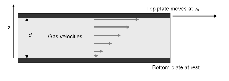
Suppose now we repeat Newton’s suggested experiment, the two parallel plates with one at rest the other moving at steady speed, but with gas rather than liquid between the plates.
It is found experimentally that the equation still describes the force necessary to maintain steady motion, but, not surprisingly, for gases anywhere near atmospheric pressure the coefficient of viscosity is far lower than that for liquids (not counting liquid heliuma special case):
| Gas | Viscosity in 10-6 mPa.s |
|---|---|
| Air at 100K | 7.1 |
| Air at 300K | 18.6 |
| Air at 400K | 23.1 |
| Hydrogen at 300K | 9.0 |
| Helium at 300K | 20.0 |
| Oxygen at 300K | 20.8 |
| Xenon at 300K | 23.2 |
These values are from the CRC Handbook, 85th Edition, 6-201.
Note first that, in contrast to the liquid case, gas viscosity increases with temperature. Even more surprising, it is found experimentally that over a very wide range of densities, gas viscosity is independent of the density of the gas!
Returning to the two plates, and picturing the gas between as made up of layers moving at different speeds as before.
The first thing to realize is that at atmospheric pressure the molecules take up something like a thousandth of the volume of the gas. The previous picture of crowded molecules jostling each other is completely irrelevant! As we shall discuss in more detail later, the molecules of air at room temperature fly around at about 500 meters per second, the molecules have diameter around 0.35 nm, are around 3 or 4 nm apart on average, and travel of order 70 nm between collisions with other molecules.
So where does the gas viscosity come from? Think of two adjacent layers of gas moving at different speeds. Molecules from the fast layer fly into the slow layer, where after a collision or two they are slowed to go along with the rest. At the same time, some slower molecules fly into the fast layer. Even if we assume that kinetic energy is conserved in each individual molecular collision (so we’re ignoring for the moment excitation of internal modes of the molecules) the macroscopic kinetic energy of the layers of gas decreases overall (see the exercise in the preceding section). How can that be? Isn’t energy conserved? Yes, total energy is conserved, what happens is that some of the macroscopic kinetic energy of the gas moving as a smooth substance has been transferred into the microscopic kinetic energy of the individual molecules moving in random directions within the gas, in other words, into the random molecular kinetic energy we call heat.
Estimating the Coefficient of Viscosity for a Gas: Momentum Transfer and Mean Free Path
The way to find the viscosity of a gas is to calculate the rate of -direction (downward) transfer of -momentum, as explained in the previous section but one.
The moving top plate maintains a steady horizontal flow pattern, the -direction speed at height
As explained above, the moving plate is feeding -direction momentum into the gas at a rate this momentum moves down through the gas at a steady rate, and the coefficient of viscosity tells us what this rate of momentum flow is for a given velocity gradient.
In fact, this rate of momentum flow can be calculated from a simple kinetic picture of the gas: remember the molecules have about a thousand times more room than they do in the liquid state, so the molecules go (relatively) a long way between collisions. We shall examine this kinetic picture of a gas in much more detail later in the course, but for now we’ll make the simplifying assumption that the molecules all have speed and travel a distance between collisions. Actually this approximation gets us pretty close to the truth.
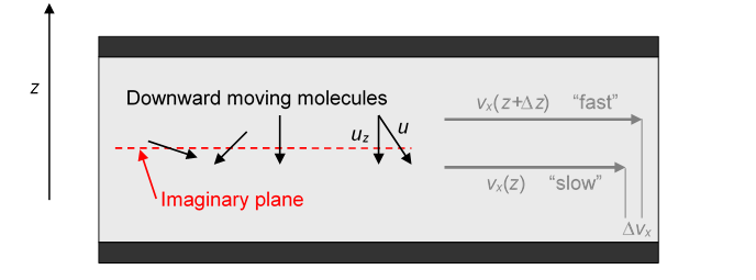
We take the density of molecules to be the molecular mass To begin thinking about -direction momentum moving downwards, imagine some plane parallel to the plates and between them. Molecules from above are shooting through this plane and colliding with molecules in the slower moving gas below, on average transferring a little extra momentum in the -direction to the slower stream. At the same time, some molecules from the slower stream are shooting upwards and will slow down the faster stream.
Let’s consider first the molecules passing through the imaginary plane from above: we’re only interested in the molecules already moving downwards, that’s half of them, so a molecular density of If we assume for simplicity that all the molecules move at the same speed then the average downward speed of these molecules ( and the average value of over all downward pointing directions is )
Thus the number of molecules per second passing through the plane from above is
and the same number are of course coming up from below! (Not shown.) (To see what’s going on, the mean free path shown here is hugely exaggerated compared with the distance between the plates, of course.)
But this isn’t quite what we want: we need to know how efficiently these molecules crossing the plane are transferring momentum for the fast moving streams above to the slower ones below. Consider one particular molecule going from the faster stream at some downward angle into the slower stream.
Let us assume it travels a distance from its last collision in the “fast” stream to its first in the “slow” stream. The average distance between collisions is called the mean free path, here “mean” is used in the sense of “average”, and we'll write the mean free path We're simplifying slightly by taking all distances between collisions to be l, so we don’t bother with statistical averaging of the distance traveled. This does not make a big difference. The distance traveled in the downward direction is , so the ( -direction) speed difference between the two streams is
The molecule has mass so on average the momentum transferred from the fast stream to the slow stream is With our simplifying assumption that all molecules have the same speed all downward values of between 0 and u are equally likely, and the density of downward-moving molecules is so the rate of transfer of momentum by downward-moving molecules through the plane is
At the same time, molecules are moving upwards form the slower streams into the faster ones, and the calculation is exactly the same. These two processes have the same sign: in the first case, the slower stream is gaining forward momentum from the faster, in the second, the faster stream is losing forward momentum, and in both cases total forward momentum is conserved. Therefore, the two processes make the same contribution, and the total momentum flow rate (per unit area) across the plane is
using
Evidently this rate of downward transfer of -direction momentum doesn’t depend on what level between the plates we choose for our imaginary plane, it’s the same momentum flow all the way from the top plate to the bottom plate: so it’s simply the rate at which the moving top plate is supplying -direction momentum to the fluid,
Since the momentum supplied moves steadily downwards through the fluid, the supply rate is the transfer rate, the two equations above are for the same thing, and we deduce that the coefficient of viscosity
It should be noted that the in the above equation is the mean speed of the atoms or molecules, which is about 8% greater than the rms speed appearing in the formula for gas pressure. In deriving the formula, we did make the simplifying assumption that all the molecules move at the same speed, and had the same mean free path, but Maxwell showed in 1860 that a more careful treatment gives essentially the same result. As discussed below, this result was historically important because when put together with other measurements, in particular the van der Waals isotherms for real gases, it led to estimates of the sizes of atoms. A great deal of effort has been expended improving Maxwell’s formula. Maxwell assumed that after a collision, the molecules recoiled in random directions. In fact, a fast-moving molecule will tend to be deflected less, so fast-moving downward molecules will have effectively longer mean free paths than slow-moving ones, and this will substantially increase the viscosity over that predicted using the “slow” mean free path. Further progress can be made if the interaction between molecules is represented by a definite potential, so the scattering can be analyzed in detail. From measurements of viscosity as a function of density, it is then possible to learn something about the actual intermolecular potential.
Why Doesn’t the Viscosity of a Gas Depend on Density?
Imagine we have a gas made up of equal numbers of red and green molecules, which have the same size, mass, etc. One of the molecules traveling through will on average have half its collisions with red molecules, half with green. If now all the red molecules suddenly disappear, the collision rate for our wandering molecule will be halved. This means its mean free path will double. So, since the coefficient of viscosity halving the gas number density at the same time doubles the mean free path so is unchanged. ( does finally begin to drop when there is so little gas left that the mean free path is of order the size of the container.)
Another way to see this is to think about the molecules shooting down from the faster stream into slower streams in the two-plate scenario. If the density is halved, there will only be half the molecules moving down, but each will deliver the -momentum difference twice as farthe further they go, the bigger the -velocity difference between where they begin and where they end, and the more effective they are in transporting -momentum downwards.
Comparing the Viscosity Formula with Experiment
We’ll repeat the earlier table here for convenience:
| Gas | Viscosity in 10-6 mPa.s |
|---|---|
| Air at 100K | 7.1 |
| Air at 300K | 18.6 |
| Air at 400K | 23.1 |
| Hydrogen at 300K | 9.0 |
| Helium at 300K | 20.0 |
| Oxygen at 300K | 20.8 |
| Xenon at 300K | 23.2 |
These values are from the CRC Handbook, 85th Edition, 6-201.
It’s easy to see one reason why the viscosity increases with temperature: from is proportional to the average molecular speed and since this depends on temperature as (if this is unfamiliar, be assured we’ll be discussing it in detail later), this factor contributes a dependence. In fact, though, from the table above, the increase in viscosity with temperature is more rapid than . We know the density and mass remain constant (we’re far from relativistic energies!) so if the analysis is correct, the mean free path must also be increasing with temperature. In fact this is what happensmany of the changes of molecular direction in flight are not caused by hard collisions with other molecules, but by longer range attractive forces (van der Waals forces) when one molecule simply passes reasonably close to another. Now these attractive forces obviously act for a shorter time on a faster molecule, so it is deflected less. This means that as temperature and molecular speed increase, the molecules get further in approximately the same direction, and therefore transport momentum more effectively.
Comparing viscosities of different gases, at the same temperature and pressure they will have the same number density (Recall that a mole of any gas has Avogadro’s number of molecules, and that at standard temperature and pressure this occupies 22.4 liters, for any gas, if tiny pressure and volume corrections for molecular attraction and molecular volume are ignored.) The molecules will also have the same kinetic energy since they’re at the same temperature (see previous paragraph).
Comparing hydrogen with oxygen, for example, the molecular mass is up by a factor 16 but the velocity decreases by a factor 4 (since the molecular kinetic energies are the same at the same temperature). In fact (see the table above), the viscosity of oxygen is only twice that of hydrogen, so from we conclude that the hydrogen molecule has twice the mean free path distance between collisionsnot surprising since it is smaller. Also, helium must have an even longer mean free path, again not surprising for the smallest molecule in existence. The quite large difference between nitrogen and oxygen, next to each other in the periodic table, is because N2 has a trivalent bonding, tighter than the divalent O2 bonding, and in fact the internuclear distance in the N2 molecule is 10% less than in O2. Xenon is heavy (atomic weight 131), but its mean free path is shorter than the others because the atom is substantially larger, and so an easier target.
Historically, the sizes of many atoms and molecules were first estimated from viscosity measurements using this method. In fact, just such a table of atomic and molecular diameters, calculated on the assumption that the atoms or molecules are hard spheres, can be found in the CRC tables. But the true picture is more complicated: the atoms are not just hard spheres, as mentioned earlier they have van der Waals attractive forces between them, beyond the outermost shell. Actually, the electronic densities of atoms and molecules can now be found fairly precisely by quantum calculations, and the resulting “radii” are in reasonable agreement with those deduced from viscosity (there is no obvious natural definition of radius for the electron cloud).
More General Laminar Flow Velocity Distributions
We’ve analyzed a particularly simple case: for the fluid between two parallel plates, the bottom plate at rest and the top moving at steady speed the fluid stream velocity increases linearly from zero at the bottom to at the top. For more realistic laminar flow situations, such as that away from the banks in a wide river, or flow down a pipe, the rate of velocity increase on going from the fixed boundary (river bed or pipe surface) into the fluid is no longer linear, that is, is not the same everywhere.
The key to analyzing these more general laminar flow patterns is to find the forces acting on a small area of one of the “sheets”. (Or a larger area of sheet if the flow is uniform in the appropriate direction.) There will be external forces such as gravity or pressure maintaining the flow, which must balance the viscous drag forces exerted by neighboring sheets if the fluid is not accelerating. The sheet-sheet drag force is equivalent to the force exerted by the top “sheet” of fluid on the top plate in the previous discussion, except that now the forces are within the fluid. As we discussed earlier, the drag force on the top plate comes from molecules close to the plate bouncing off, gaining momentum, which is subsequently transferred to other molecules a little further away. For liquids, this mechanism involves distances of order a few molecular diameters, for gases a few mean free paths. In either case, the distances are tiny on a macroscopic scale. This means that the appropriate formula for the drag force on a plate, or that between one sheet of fluid on another, is
The rate of change of stream velocity close to the interface determines the drag force.
We shall show in the next lecture how this formula can be used to determine the flow pattern in a river, and that in a circular pipe.