previous (simple harmonic oscillator) index next (critical damping)

Oscillations I: Heavily Damped Oscillator

Michael Fowler

Introduction

In the next three lectures, we'll look at a wide variety of oscillatory phenomena. After a brief recap of undamped simple harmonic motion, we analyze the motion of a heavily damped oscillator. Why start with that? Well, the math is very straightforward (no complex numbers) and there is some nontrivial physics. Following that, we'll cover the lightly damped oscillator, where we do need complex numbers—avoiding them leads to very cumbersome trigonometry. We'll also discuss the important intermediate case called critical damping. Finally, in the third lecture, we examine the physically very relevant case of a driven damped oscillator—and when that leads to disaster.

Applets

We have a set of easy-to-use applets illustrating these oscillators—and it's a great way to get a feel for the subject! If you're already pretty familiar with simple harmonic motion, you can skip or just glance through the next section, and begin exploring the heavily damped oscillator with this applet.

Brief Review of Undamped Simple Harmonic Motion

Our basic model simple harmonic oscillator is a mass $m$ moving back and forth along a line on a smooth horizontal surface, connected to an inline horizontal spring, having spring constant $k,$ the other end of the string being attached to a wall. The spring exerts a restoring force equal to $- k x,$ on the mass when it is a 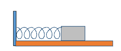distance $x$ from the equilibrium point. By “equilibrium point” we mean the point corresponding to the spring resting at its natural length, and therefore exerting no force on the mass. The in-class realization of this model was an aircar, with a light spring above the track (actually, we used two light springs, going in opposite directions $—$ we found if we just one it tended to sag on to the track when it was slack, but two in opposite directions could be kept taut. The two springs together act like a single spring having spring constant the sum of the two).

Newton’s Law gives:

$F = m a, or m \frac{d^{2} x}{d t^{2}} = - k x .$

Solving this differential equation gives the position of the mass (the aircar) relative to the rest position as a function of time:

$x (t) = A \cos (ω_{0} t + φ) .$

Here $A$ is the maximum displacement, and is called the amplitude of the motion. $ω_{0} t + φ$ is called the phase. $φ$ is called the phase constant: it depends on where in the cycle you start, that is, where is the oscillator at time zero.

The velocity and acceleration are given by differentiating $x (t)$ once and twice:

$v (t) = \frac{d x}{d t} = - A ω_{0} \sin (ω_{0} t + φ)$

and

$a (t) = \frac{d^{2} x (t)}{d t^{2}} = - A ω_{0}^{2} \cos (ω_{0} t + φ) .$

We see immediately that this $x (t)$ does indeed satisfy Newton’s Law provided $ω_{0}$ is given by

$ω_{0} = \sqrt{k / m} .$

Exercise: Verify that, apart from a possible overall constant, this expression for $ω_{0}$ could have been figured out using dimensions.

Energy Conservation in Undamped Simple Harmonic Motion

The spring stores potential energy: if you push one end of the spring from some positive extension $x$ to $x + d x$ (with the other end of the spring fixed, of course) the force $- k x$ opposes the motion, so you must push with force $+ k x,$ and therefore do work $k x d x .$ To find the total potential energy stored by the spring when the end is $x_{0}$ away from the equilibrium point (the natural spring length) we must find the total work required to stretch the spring from that resting length to an extension $x_{0} .$ This means adding up all the little bits of work $k x d x$ needed to get the spring from no extension at all to an extension of $x_{0} .$ In other words, we need to do an integral to find the potential energy $U (x_{0}) :$

_{$U (x_{0}) = \int_{0}^{x_{0}} k x d x = \frac{1}{2} k x_{0}^{2} .$}

So the potential energy plotted as a function of distance from equilibrium is parabolic:

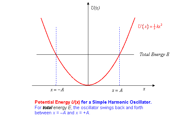
The oscillator has total energy equal to kinetic energy + potential energy,

$E = \frac{1}{2} m v^{2} + \frac{1}{2} k x^{2}$

when the mass is at position $x .$ Putting in the values of $x (t), v (t)$ from the equations above, it is easy to check that $E$ is independent of time and equal to $\frac{1}{2} k A^{2}, A$ being the amplitude of the motion, the maximum displacement. Of course, when the oscillator is at $x = \pm A,$ it is momentarily at rest, so has no kinetic energy.

Heavily Damped Oscillator: Pendulum in Molasses

Once we allow damping, it turns out that heavy damping is a little easier to deal with than light damping, so we'll look at this first. (When, exactly, does damping count as heavy? We'll see shortly.)

Suppose, then, the oscillator is subject to a drag force proportional to velocity.

The equation of motion is:

$m \frac{d^{2} x}{d t^{2}} = - k x - b \frac{d x}{d t} .$

Although this equation looks much more difficult than the no-drag case, it really isn’t!

The important point is that the terms are just derivatives of $x$ with respect to time, multiplied by constants. The math would be a lot more difficult if we had a drag force proportional to the square of the velocity, or if the force exerted by the spring were not a constant times $x$ (this means we can’t stretch the string too far $—$ they all go nonlinear for a big enough stretch). Anyway, it is easy to find exponential functions that are solutions to this equation. Let us guess a solution:

$x = x_{0} e^{- α t} .$

We're guessing that, thanks to the molasses it won't actually oscillate. Can that be right? We'll find out. Inserting this proposed solution in the equation of motion, using

$\frac{d x}{d t} = - α x_{0} e^{- α t}, \frac{d^{2} x}{d t^{2}} = α^{2} x_{0} e^{- α t}$

we find that it is a valid solution provided that $α$ satisfies:

$m α^{2} - α b + k = 0$

from which

$α = \frac{b \pm \sqrt{b^{2} - 4 m k}}{2 m} .$

Staring at this expression for $α$ , we notice that for $α$ to be real, we need to have

$b^{2} > 4 m k .$

What can that mean? Remember $b$ is the damping parameter $—$ we’re finding that our proposed exponential solution only works for large damping! (We know physically, of course, that if the damping is small, the pendulum will swing, a motion not described by our exponential decay function.) We'll analyze the large damping case now, then after that go on to see how to extend the solution to small damping.

Interpreting the Two Different Exponential Solutions

If you haven't already done so, at this point pull up the applet and look through the suggestions.

It’s worth looking at the case of very large damping (imagine our mass and spring being in a tub of molasses), where the two exponential solutions turn out to decay at very different rates. For $b^{2}$ much greater than $4 m k,$ we can write

$α = \frac{b \pm b \sqrt{1 - \frac{4 m k}{b^{2}}}}{2 m} = α_{1}, α_{2}$

and then expand the square root using

${(1 - x)}^{1 / 2} ≅ 1 - \frac{1}{2} x,$

valid for small $x,$ to find that approximately $—$ for large $b$ $—$ the two possible values of $α$ are:

$α_{1} = \frac{b}{m} and α_{2} = \frac{k}{b} .$

That is to say, there are two possible highly damped decay modes,

$x = A_{1} e^{- α_{1} t} and x = A_{2} e^{- α_{2} t} .$

Note that since the damping $b$ is large, $α_{1}$ is large, meaning fast decay, and $α_{2}$ is small, meaning slow decay.

Question: what, physically, is going on in these two different highly damped exponential decays? Here's a picture of two identical oscillators, with the same damping, generated by the applet: 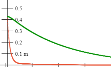Can you reconstruct it using the applet, and explain physically why two very different rates of change of speed are possible?

Hint: look again at the equation of motion of the damped oscillator. Notice that in each of these highly damped decays, one term doesn’t play any part $—$ but the irrelevant term is a different term for the two decays!

Answer 1: for $α = k / b$ , evidently the mass doesn’t play a role. This decay is what you get if you pull the mass to one side, let go, then, after it gets moving, it will very slowly settle towards the equilibrium point. Its rate of approach is determined by balancing the spring’s force against the speed-dependent damping force, to give the speed. The rate of change of speed $—$ the acceleration $—$ is so tiny that the inertial term $—$ the mass $—$ is negligible.

Answer 2: for $α = b / m$ , the spring is negligible. And, this is very fast motion ( $b / m ≫ k / b,$ since we said $b^{2} ≫ 4 m k .$ ) The way to get this motion is to pull the mass to one side, then give it a very strong kick towards the equilibrium point. If you give it just the right (high) speed, all the momentum you imparted will be spent overcoming the damping force as the mass moves to the center $—$ the force of the spring will be negligible.

*The Most General Solution for the Highly Damped Oscillator

The damped oscillator equation

$m \frac{d^{2} x}{d t^{2}} = - k x - b \frac{d x}{d t}$

is a linear equation. This means that if $x_{1} (t)$ is a solution, and $x_{2} (t)$ is another solution, that is,

$\begin{array}{l} m \frac{d^{2} x_{1} (t)}{d t^{2}} = - k x_{1} (t) - b \frac{d x_{1} (t)}{d t} \\ m \frac{d^{2} x_{2} (t)}{d t^{2}} = - k x_{2} (t) - b \frac{d x_{2} (t)}{d t} \end{array}$

then just adding the two equations we get:

_{$m \frac{d^{2} (x_{1} (t) + x_{2} (t))}{d t^{2}} = - k (x_{1} (t) + x_{2} (t)) - b \frac{d (x_{1} (t) + x_{2} (t))}{d t} .$}

It is also clear that multiplying a solution by a constant produces another solution: if $x (t)$ satisfies the equation, so does $3 x (t) .$

This means, then, that given two solutions $x_{1} (t)$ and $x_{2} (t),$ and two arbitrary constants $A_{1}$ and $A_{2},$ the function

$A_{1} x_{1} (t) + A_{2} x_{2} (t)$

is also a solution of the differential equation.

In fact, all possible motions of the highly damped oscillator have this form. The way to understand this is to realize that the oscillator’s motion is completely determined if we specify at an initial instant of time both the position and the velocity of the oscillator. The equation of motion gives the acceleration as a function of position and velocity, so, at least in principle, we can work out step by step how the mass must move; technically, we are integrating the equation of motion, either mathematically, or numerically such as by using Mathematica or a spreadsheet. So, by suitably adjusting the two arbitrary constants $A_{1}$ and $A_{2},$ we can match our sum of solutions to any given initial position and velocity.

To summarize, for the highly damped oscillator any solution is of the form:

$x (t) = A_{1} e^{- α_{1} t} + A_{2} e^{- α_{2} t} = A_{1} e^{- \frac{b + b \sqrt{1 - \frac{4 m k}{b^{2}}}}{2 m} t} + A_{2} e^{- \frac{b - b \sqrt{1 - \frac{4 m k}{b^{2}}}}{2 m} t} .$

Exercises on highly damped oscillations

1. If the oscillator is pulled aside a distance $x_{0},$ and released from rest at $t = 0,$ what are $A_{1}, A_{2}$ ? Describe the subsequent motion, especially the very beginning: what is the initial acceleration? Hint: think carefully about how important the damping term is immediately after release from rest $—$ you should be able to guess the initial acceleration. Look at this graph from 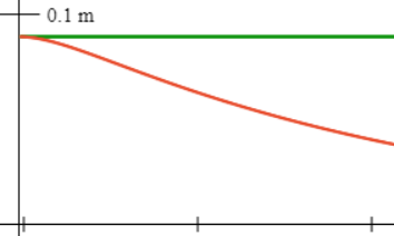the applet, we set one spring equal to zero.

2. If the oscillator is initially at the equilibrium position $x_{0} = 0,$ but is given a kick to a velocity $v_{0},$ find $A_{1}$ and $A_{2}$ and describe the subsequent motion.

*The Principle of Superposition for Linear Differential Equations

The equation for the highly damped oscillator is a linear differential equation, that is, an equation of the form (in more usual notation):

$c_{0} f (x) + c_{1} \frac{d f (x)}{d x} + c_{2} \frac{d^{2} f (x)}{d x^{2}} = 0$

where $c_{0}, c_{1}$ and $c_{2}$ are constants, that is, independent of $x .$

For such a linear differential equation, if $f_{1} (x)$ and $f_{2} (x)$ are solutions, so is $A_{1} f_{1} (x) + A_{2} f_{2} (x)$ for any constants $A_{1}, A_{2} .$

This is called the Principle of Superposition, and is proved in general exactly as we proved it for the highly damped oscillator in the preceding section.

Even more important, this Principle of Superposition is valid, using analogous arguments, for linear differential equations in more than one variable, such as the wave equations we'll be considering shortly. In that case, it gives insight into how waves can pass through each other and emerge unchanged.

previous index next