Physics 252: Modern Physics! previous index next Physics 152: previous index next

Kinetic Theory of Gases: A Brief Review

Michael Fowler

Bernoulli's Picture

Daniel Bernoulli, in 1738, was the first to understand air pressure from a molecular point of view. He drew a picture of a vertical cylinder, closed at the bottom, with a piston at the top, the piston having a weight on it, both piston and weight being supported by the air pressure inside the cylinder.

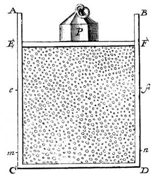
He described what went on inside the cylinder as follows: “let the cavity contain very minute corpuscles, which are driven hither and thither with a very rapid motion; so that these corpuscles, when they strike against the piston and sustain it by their repeated impacts, form an elastic fluid which will expand of itself if the weight is removed or diminished…”

Sad to report, his insight, although essentially correct, was not widely accepted. Most scientists believed that the molecules in a gas stayed more or less in place, repelling each other from a distance, held somehow in the ether. Newton had shown that $P V =$ constant followed if the repulsion were inverse-square. In fact, in the 1820’s an Englishman, John Herapath, derived the relationship between pressure and molecular speed given below, and tried to get it published by the Royal Society. It was rejected by the president, Humphry Davy, who pointed out that equating temperature with motion, as Herapath did, implied that there would be an absolute zero of temperature, an idea Davy was reluctant to accept. And it should be added that no-one had the slightest idea how big atoms and molecules were, although Avogadro had conjectured that equal volumes of different gases at the same temperature and pressure contained equal numbers of molecules $—$ his famous number $—$ neither he nor anyone else knew what that number was, only that it was pretty big.

The Link between Molecular Energy and Pressure

It is not difficult to extend Bernoulli’s picture to a quantitative description, relating the gas pressure to the molecular velocities. As a warm up exercise, let us consider a single perfectly elastic particle, of mass $m,$ bouncing rapidly back and forth at speed $v$ inside a narrow cylinder of length $L$ with a piston at one end, so all motion is along the same line. (For the movie, click here!) What is the force on the piston?

Obviously, the piston doesn’t feel a smooth continuous force, but a series of equally spaced impacts. However, if the piston is much heavier than the particle, this will have the same effect as a smooth force over times long compared with the interval between impacts. So what is the value of the equivalent smooth force?

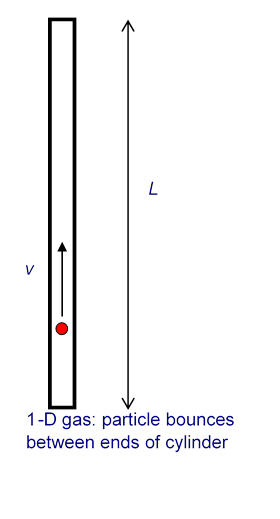
Using Newton’s law in the form force = rate of change of momentum, we see that the particle’s momentum changes by $2 m v$ each time it hits the piston. The time between hits is $2 L / v,$ so the frequency of hits is $v / 2 L$ per second. This means that if there were no balancing force, by conservation of momentum the particle would cause the momentum of the piston to change by $2 m v \times v / 2 L$ units in each second. This is the rate of change of momentum, and so must be equal to the balancing force, which is therefore $F = m v^{2} / L .$

We now generalize to the case of many particles bouncing around inside a rectangular box, of length $L$ in the $x$ -direction (which is along an edge of the box). The total force on the side of area $A$ perpendicular to the $x$ -direction is just a sum of single particle terms, the relevant velocity being the component of the velocity in the $x$ -direction. The pressure is just the force per unit area, $P = F / A .$ Of course, we don’t know what the velocities of the particles are in an actual gas, but it turns out that we don’t need the details. If we sum $N$ contributions, one from each particle in the box, each contribution proportional to $v_{x}^{2}$ for that particle, the sum just gives us $N$ times the average value of $v_{x}^{2} .$ That is to say,

$P = F / A = N m \bar{v_{x}^{2}} / L A = N m \bar{v_{x}^{2}} / V$

where there are $N$ particles in a box of volume $V .$ Next we note that the particles are equally likely to be moving in any direction, so the average value of $v_{x}^{2}$ must be the same as that of $v_{y}^{2}$ or $v_{z}^{2},$ and since $v^{2} = v_{x}^{2} + v_{y}^{2} + v_{z}^{2},$ it follows that

$P = N m \bar{v^{2}} / 3 V .$

This is a surprisingly simple result! The macroscopic pressure of a gas relates directly to the average kinetic energy per molecule.

Of course, in the above we have not thought about possible complications caused by interactions between particles, but in fact for gases like air at room temperature these interactions are very small. Furthermore, it is well established experimentally that most gases satisfy the Gas Law over a wide temperature range:

$P V = n R T$

for $n$ n moles of gas, that is, $n = N / N_{A},$ with $N_{A}$ Avogadro’s number and $R$ the gas constant.

Introducing Boltzmann’s constant $k_{B} = R / N_{A},$ it is easy to check from our result for the pressure and the ideal gas law that the average molecular kinetic energy is proportional to the absolute temperature,

$\bar{E_{K}} = \bar{\frac{1}{2} m v^{2}} = \frac{3}{2} k_{B} T .$

Boltzmann’s constant $k_{B} =$ 1.38.10^-23 joules/K.

Maxwell finds the Velocity Distribution

By the 1850’s, various difficulties with the existing theories of heat, such as the caloric theory, caused some rethinking, and people took another look at the kinetic theory of Bernoulli, but little real progress was made until Maxwell attacked the problem in 1859. Maxwell worked with Bernoulli’s picture, that the atoms or molecules in a gas were perfectly elastic particles, obeying Newton’s laws, bouncing off each other (and the sides of the container) with straight-line trajectories in between collisions. (Actually, there is some inelasticity in the collisions with the sides—the bouncing molecule can excite or deexcite vibrations in the wall, this is how the gas and container come to thermal equilibrium.) Maxwell realized that it was completely hopeless to try to analyze this system using Newton’s laws, even though it could be done in principle, there were far too many variables to begin writing down equations. On the other hand, a completely detailed description of how each molecule moved was not really needed anyway. What was needed was some understanding of how this microscopic picture connected with the macroscopic properties, which represented averages over huge numbers of molecules.

The relevant microscopic information is not knowledge of the position and velocity of every molecule at every instant of time, but just the distribution function, that is to say, what percentage of the molecules are in a certain part of the container, and what percentage have velocities within a certain range, at each instant of time. For a gas in thermal equilibrium, the distribution function is independent of time. Ignoring tiny corrections for gravity, the gas will be distributed uniformly in the container, so the only unknown is the velocity distribution function.

To see easily how random collisions can produce a well-defined velocity distribution, even if we start with all the molecules having the same speed, check out this applet!

Velocity Space

What does a velocity distribution function look like? Suppose at some instant in time one particular molecule has velocity $\vec{v} = (v_{x}, v_{y}, v_{z}) .$ We can record this information by constructing a three-dimensional velocity space, with axes $v_{x}, v_{y}, v_{z},$ and putting in a point $P_{1}$ P₁ representing the molecule’s velocity (the red arrow is of course $\vec{v}$ ):

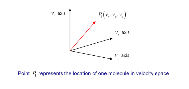
Now imagine that at that instant we could measure the velocities of all the molecules in a container, and put points $P_{2}, P_{3}, P_{4}, \dots, P_{N}$ in the velocity space. Since $N$ is of order 10²¹ for 100 ccs of gas, this is not very practical! But we can imagine what the result would be: a cloud of points in velocity space, equally spread in all directions (there’s no reason molecules would prefer to be moving in the $x$ -direction, say, rather than the $y$ -direction) and thinning out on going away from the origin towards higher and higher velocities.

Now, if we could keep monitoring the situation as time passes individual points would move around, as molecules bounced off the walls, or each other, so you might think the cloud would shift around a bit. But there’s a vast number of molecules in any realistic macroscopic situation, and for any reasonably sized container it’s safe to assume that the number of molecules in any small region of velocity space remains pretty much constant. Obviously, this cannot be true for a region of velocity space so tiny that it only contains one or two molecules on average. But it can be shown statistically that if there are $N$ molecules in a particular small volume of velocity space, the fluctuation of the number with time is of order $\sqrt{N},$ so a region containing a million molecules will vary in numbers by about one part in a thousand, a trillion molecule region by one part in a million. Since 100 ccs of air contains of order 10²¹ molecules, we can in practice divide the region of velocity space occupied by the gas into a billion cells, and still have variation in each cell of order one part in a million!

The bottom line is that for a macroscopic amount of gas, fluctuations in density, both in ordinary space and in velocity space, are for all practical purposes negligible, and we can take the gas to be smoothly distributed in both spaces.

Maxwell’s Symmetry Argument

Maxwell found the velocity distribution function for gas molecules in thermal equilibrium by the following elegant argument based on symmetry.

For a gas of $N$ particles, let the number of particles having velocity in the $x$ -direction between $v_{x}$ and $v_{x} + d v_{x}$ be $N f_{1} (v_{x}) d v_{x} .$ In other words, $f_{1} (v_{x}) d v_{x}$ is the fraction of all the particles having $x$ -direction velocity lying in the interval between $v_{x}$ and $v_{x} + d v_{x} .$ (I’ve written $f_{1}$ instead of $f$ to help remember this function refers to only one component of the velocity vector.)

If we add the fractions for all possible values of $v_{x},$ the result must of course be 1:

$\int_{- \infty}^{\infty} f_{1} (v_{x}) d v_{x} = 1.$

But there’s nothing special about the $x$ -direction $—$ for gas molecules in a container, at least away from the walls, all directions look the same, so the same function $f$ will give the probability distributions in the other directions too. It follows immediately that the probability for the velocity to lie between $v_{x}$ and $v_{x} + d v_{x}$ , $v_{y}$ and $v_{y} + d v_{y},$ and $v_{z}$ and $v_{z} + d v_{z}$ must be:

$N f_{1} (v_{x}) d v_{x} f_{1} (v_{y}) d v_{y} f_{1} (v_{z}) d v_{z} = N f_{1} (v_{x}) f_{1} (v_{y}) f_{1} (v_{z}) d v_{x} d v_{y} d v_{z} .$

Note that this distribution function, when integrated over all possible values of the three components of velocity, gives the total number of particles to be $N,$ as it should (since integrating over each $f_{1} (v) d v$ gives unity).

Next comes the clever part $—$ since any direction is as good as any other direction, the distribution function must depend only on the total speed of the particle, not on the separate velocity components. Therefore, Maxwell argued, it must be that:

$f_{1} (v_{x}) f_{1} (v_{y}) f_{1} (v_{z}) = F (v_{x}^{2} + v_{y}^{2} + v_{z}^{2})$

where $F$ is another unknown function. However, it is apparent that the product of the functions on the left is reflected in the sum of variables on the right. It will only come out that way if the variables appear in an exponent in the functions on the left. In fact, it is easy to check that this equation is solved by a function of the form:

$f_{1} (v_{x}) = A e^{- B v_{x}^{2}} .$

This curve is called a Gaussian: it’s centered at the origin, and falls off very rapidly as $v_{x}$ increases. Taking $A = B = 1$ just to see the shape, we find:

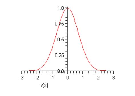
At this point, $A$ and $B$ are arbitrary constants $—$ we shall eventually find their values for an actual sample of gas at a given temperature. Notice that (following Maxwell) we have put a minus sign in the exponent because there must eventually be fewer and fewer particles on going to higher speeds, certainly not a diverging number.

Multiplying together the probability distributions for the three directions gives the distribution in terms of particle speed $v,$ where $v^{2} = v_{x}^{2} + v_{y}^{2} + v_{z}^{2} .$ Since all velocity directions are equally likely, it is clear that the natural distribution function is that giving the number of particles having speed between $v$ and $v + d v .$

From the graph above, it is clear that the most likely value of $v_{x}$ is zero. If the gas molecules were restricted to one dimension, just moving back and forth on a line, then the most likely value of their speed would also be zero. However, for gas molecules free to move in two or three dimensions, the most likely value of the speed is not zero. It’s easiest to see this in a two-dimensional example. Suppose we plot the points P representing the velocities of molecules in a region near the origin, so the density of points doesn’t vary much over the extent of our plot (we’re staying near the top of the peak in the one-dimensional curve shown above).

Now divide the two-dimensional space into regions corresponding to equal increments in speed:

$0 to Δ v, Δ v to 2 Δ v, 2 Δ v to 3 Δ v, \dots$

In the two-dimensional space, $v = \sqrt{v_{x}^{2} + v_{y}^{2}} = constant$ is a circle, so this division of the plane is into annular regions between circles whose successive radii are $Δ v$ apart:

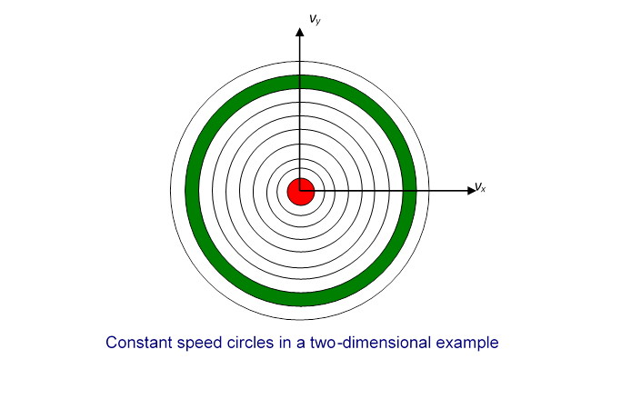
Each of these annular areas corresponds to the same speed increment $Δ v .$ In particular, the green area, between a circle of radius $8 Δ v$ and one of radius $9 Δ v,$ corresponds to the same speed increment as the small red circle in the middle, which corresponds to speeds between 0 and $Δ v .$ Therefore, if the molecular speeds are pretty evenly distributed in this near-the-origin area of the $(v_{x}, v_{y})$ plane, there will be a lot more molecules with speeds between $8 Δ v$ and $9 Δ v$ than between 0 and $Δ v$ $—$ so the most likely speed will not be zero. To find out what it actually is, we have to put this area argument together with the Gaussian fall off in density on going far from the origin. We’ll discuss this shortly.

The same argument works in three dimensions $—$ it’s just a little more difficult to visualize. Instead of concentric circles, we have concentric spheres. All points lying on a spherical surface centered at the origin correspond to the same speed.

Let us now figure out the distribution of particles as a function of speed. The distribution in the three-dimensional space $(v_{x}, v_{y}, v_{z})$ is from Maxwell’s analysis

$\begin{matrix} # of particles in small box d v_{x} d v_{y} d v_{z} = N f_{1} (v_{x}) f_{1} (v_{y}) f_{1} (v_{z}) d v_{x} d v_{y} d v_{z} \\ = N A^{3} e^{- B (v_{x}^{2} + v_{y}^{2} + v_{z}^{2})} d v_{x} d v_{y} d v_{z} \\ = N A^{3} e^{- B v^{2}} d v_{x} d v_{y} d v_{z} \end{matrix}$

To translate this to the number of particles having speed between $v$ and $v + d v$ we need to figure out how many of those little $d v_{x} d v_{y} d v_{z}$ boxes there are corresponding to speeds between $v$ and $v + d v .$ In other words, what is the volume of velocity space between the two neighboring spheres, both centered at the origin, the inner one with radius $v,$ the outer one infinitesimally bigger, with radius $v + d v$ ? Since $d v$ is so tiny, this volume is just the area of the sphere multiplied by $d v :$ that is, $4 π v^{2} d v .$

Finally, then, the probability distribution as a function of speed is:

$f (v) d v = 4 π v^{2} A^{3} e^{- B v^{2}} d v .$

Of course, our job isn’t over $—$ we still have these two unknown constants A and B. However, just as for the function $f_{1} (v_{x}), f (v) d v$ is the fraction of the molecules corresponding to speeds between $v$ and $v + d v,$ , and all these fractions taken together must add up to 1.

That is,

$\int_{0}^{\infty} f (v) d v = 1.$

We need the standard result $\int_{0}^{\infty} x^{2} e^{- B x^{2}} d x = (1 / 4 B) \sqrt{π / B}$ (a derivation can be found in my 152 Notes on Exponential Integrals), and find:

$4 π A^{3} \frac{1}{4 B} \sqrt{\frac{π}{B}} = 1.$

This means that there is really only one arbitrary variable left: if we can find $B,$ this equation gives us $A :$ that is, $4 π A^{3} = \frac{4}{\sqrt{π}} B^{3 / 2},$ and $4 π A^{3}$ is what appears in $f (v) .$

Looking at $f (v),$ we notice that $B$ is a measure of how far the distribution spreads from the origin: if $B$ is small, the distribution drops off more slowly $—$ the average particle is more energetic. Recall now that the average kinetic energy of the particles is related to the temperature by $\bar{\frac{1}{2} m v^{2}} = \frac{3}{2} k_{B} T .$ This means that $B$ is related to the inverse temperature.

In fact, since $f (v) d v$ is the fraction of particles in the interval $d v$ at $v,$ and those particles have kinetic energy $\frac{1}{2} m v^{2},$ we can use the probability distribution to find the average kinetic energy per particle:

$\bar{\frac{1}{2} m v^{2}} = \int_{0}^{\infty} \frac{1}{2} m v^{2} f (v) d v .$

To do this integral we need another standard result: $\int_{0}^{\infty} x^{4} e^{- B x^{2}} d x = (3 / 8 B^{2}) \sqrt{π / B}$ . We find:

$\bar{\frac{1}{2} m v^{2}} = \frac{3 m}{4 B} .$

.Substituting the value for the average kinetic energy in terms of the temperature of the gas,

$\bar{\frac{1}{2} m v^{2}} = \frac{3}{2} k_{B} T$

gives $B = m / 2 k_{B} T,$ so $4 π A^{3} = \frac{4}{\sqrt{π}} B^{3 / 2} = 4 π {(\frac{m}{2 π k_{B} T})}^{3 / 2} .$

This means the distribution function

$f (v) = 4 π {(\frac{m}{2 π k_{B} T})}^{3 / 2} v^{2} e^{- m v^{2} / 2 k T} = 4 π {(\frac{m}{2 π k_{B} T})}^{3 / 2} v^{2} e^{- E / k T}$

where $E$ is the kinetic energy of the molecule.

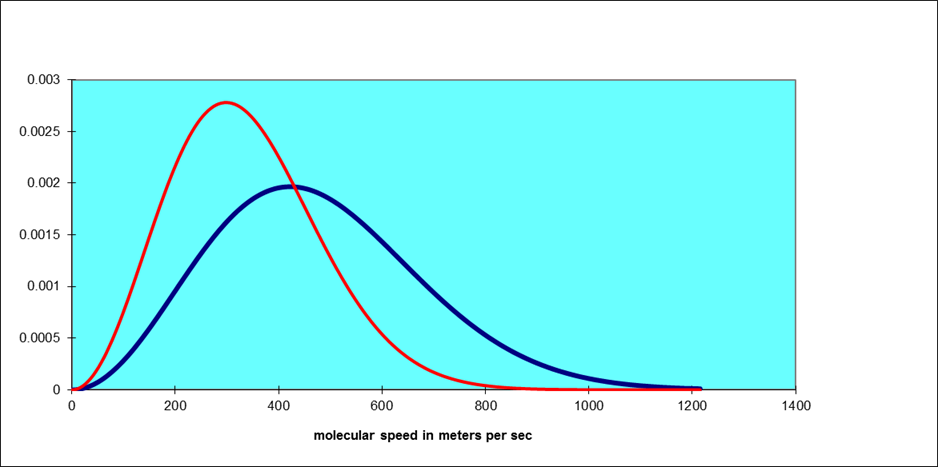
Note that this function increases parabolically from zero for low speeds, then curves round to reach a maximum and finally decreases exponentially. As the temperature increases, the position of the maximum shifts to the right. The total area under the curve is always one, by definition. For air molecules (say, nitrogen) at room temperature the curve is the blue one below. The red one is for an absolute temperature down by a factor of two:

What about Potential Energy?

Maxwell’s analysis solves the problem of finding the statistical velocity distribution of molecules of an ideal gas in a box at a definite temperature $T :$ the relative probability of a molecule having velocity $\vec{v}$ is proportional to $e^{- m v^{2} / 2 k T} = e^{- E / k T} .$ The position distribution is taken to be uniform: the molecules are assumed to be equally likely to be anywhere in the box.

But how is this distribution affected if in fact there is some kind of potential pulling the molecules to one end of the box? In fact, we’ve already solved this problem, in the discussion earlier on the isothermal atmosphere. Consider a really big box, kilometers high, so air will be significantly denser towards the bottom. Assume the temperature is uniform throughout. We found under these conditions that with Boyles Law expressed in the form

$ρ = C P$

the atmospheric density varied with height as

$P = P_{0} e^{- C g h}, or equivalently ρ = ρ_{0} e^{- C g h} .$

Now we know that Boyle’s Law is just the fixed temperature version of the Gas Law $P V = n R T,$ and the density

$ρ = mass/volume = N m / V$

with $N$ the total number of molecules and $m$ the molecular mass,

$C P = ρ = N m / V .$

Rearranging,

$P V = N m / C = n N_{A} m / C,$

for $n$ moles of gas, each mole containing Avogadro’s number $N_{A}$ molecules.

Putting this together with the Gas Law,

$P V = n N_{A} m / C = n R T,$

$C = N_{A} m / R T = m / k_{B} T$

where Boltzmann’s constant $k_{B} = R / N_{A}$ as discussed previously.

The dependence of gas density on height can therefore be written

$ρ = ρ_{0} e^{- C g h} = ρ_{0} e^{- m g h / k_{B} T} .$

The important point here is that $m g h$ is the potential energy of the molecule, and the distribution we have found is exactly parallel to Maxwell’s velocity distribution, the potential energy now playing the role that kinetic energy played in that case.

We’re now ready to put together Maxwell’s velocity distribution with this height distribution, to find out how the molecules are distributed in the atmosphere, both in velocity space and in ordinary space. In other words, in a six-dimensional space!

Our result is:

$f (x, y, z, v_{x}, v_{y}, v_{z}) = f (h, v) \propto e^{- m v^{2} / 2 k_{B} T} e^{- m g h / k T} = e^{- ((1 / 2) m v^{2} + m g h) / k_{B} T} = e^{- E / k_{B} T} .$

That is, the probability of a molecule having total energy $E$ is proportional to $e^{- E / k_{B} T} .$

This is the Boltzmann, or Maxwell-Boltzmann, distribution. It turns out to be correct for any type of potential energy, including that arising from forces between the molecules themselves.

Degrees of Freedom and Equipartition of Energy

By a “degree of freedom” we mean a way in which a molecule is free to move, and thus have energy $—$ in this case, just the $x, y$ and $z$ directions. Boltzmann reformulated Maxwell’s analysis in terms of degrees of freedom, stating that there was an average energy $\frac{1}{2} k_{B} T$ in each degree of freedom, to give total average kinetic energy $\frac{3}{2} k_{B} T,$ so the specific heat per molecule is presumable $1.5 k_{B},$ and given that $k_{B} = R / N_{A},$ the specific heat per mole comes out at $1.5 R .$ In fact, this is experimentally confirmed for monatomic gases. However, it is found that diatomic gases can have specific heats of $2.5 R$ and even $3.5 R .$ This is not difficult to understand $—$ these molecules have more degrees of freedom. A dumbbell molecule can rotate about two directions perpendicular to its axis. A diatomic molecule could also vibrate. Such a simple harmonic oscillator motion has both kinetic and potential energy, and it turns out to have total energy $k_{B} T$ in thermal equilibrium. Thus, reasonable explanations for the specific heats of various gases can be concocted by assuming a contribution $\frac{1}{2} k_{B}$ from each degree of freedom. But there are problems. Why shouldn’t the dumbbell rotate about its axis? Why do monatomic atoms not rotate at all? Even more ominously, the specific heat of hydrogen, $2.5 R$ at room temperature, drops to $1.5 R$ at lower temperatures. These problems were not resolved until the advent of quantum mechanics.

Brownian Motion

One of the most convincing demonstrations that gases really are made up of fast moving molecules is Brownian motion, the observed constant jiggling around of tiny particles, such as fragments of ash in smoke. This motion was first noticed by a Scottish botanist, who initially assumed he was looking at living creatures, but then found the same motion in what he knew to be particles of inorganic material. Einstein showed how to use Brownian motion to estimate the size of atoms. For the applet, click here!

Physics 252: Modern Physics! previous index next Physics 152: previous index next