Fourier Series, Fourier Transforms and the Delta Function

Michael Fowler, UVa.

Introduction

We begin with a brief review of Fourier series. Any periodic function of interest in physics can be expressed as a series in sines and cosines $—$ we have already seen that the quantum wave function of a particle in a box is precisely of this form. The important question in practice is, for an arbitrary wave function, how good an approximation is given if we stop summing the series after $N$ terms. We establish here that the sum after $N$ terms, $f_{N} (θ)$ , can be written as a convolution of the original function with the function

$δ_{N} (x) = (1 / 2 π) (\sin (N + \frac{1}{2}) x) / \sin \frac{1}{2} x,$

that is,

$f_{N} (θ) = \int_{- π}^{π} δ_{N} (θ - θ^{'}) f (θ^{'}) d θ^{'}$ .

The structure of the function $δ_{N} (x)$ (plotted below), when put together with the function $f (θ)$ , gives a good intuitive guide to how good an approximation the sum over $N$ terms is going to be for a given function $f (θ)$ . In particular, it turns out that step discontinuities are never handled perfectly, no matter how many terms are included. Fortunately, true step discontinuities never occur in physics, but this is a warning that it is of course necessary to sum up to some $N$ where the sines and cosines oscillate substantially more rapidly than any sudden change in the function being represented.

We go on to the Fourier transform, in which a function on the infinite line is expressed as an integral over a continuum of sines and cosines (or equivalently exponentials $e^{i k x}$ ). It turns out that arguments analogous to those that led to $δ_{N} (x)$ now give a function $δ (x)$ such that

$f (x) = \int_{- \infty}^{\infty} δ (x - x^{'}) f (x^{'}) d x^{'} .$

Confronted with this, one might well wonder what is the point of a function $δ (x)$ which on convolution with $f (x)$ gives back the same function $f (x) .$ The relevance of $δ (x)$ will become evident later in the course, when states of a quantum particle are represented by wave functions on the infinite line, like $f (x),$ and operations on them involve integral operators similar to the convolution above. Working with operations on these functions is the continuum generalization of matrices acting on vectors in a finite-dimensional space, and $δ (x)$ is the infinite-dimensional representation of the unit matrix. Just as in matrix algebra the eigenstates of the unit matrix are a set of vectors that span the space, and the unit matrix elements determine the set of dot products of these basis vectors, the delta function determines the generalized inner product of a continuum basis of states. It plays an essential role in the standard formalism for continuum states, and you need to be familiar with it!

Fourier Series

Any reasonably smooth real function $f (θ)$ defined in the interval $- π < θ \leq π$ can be expanded in a Fourier series,

$f (θ) = \frac{A_{0}}{2} + \sum_{n = 1}^{\infty} (A_{n} \cos n θ + B_{n} \sin n θ)$

where the coefficients can be found using the orthogonality condition,

$\int_{- π}^{π} \cos m θ \cos n θ d θ = π δ_{m, n}$

and the same condition for the $\sin n θ's$ to give:

$\begin{array}{l} A_{n} = \frac{1}{π} \int_{- π}^{π} f (θ) \cos n θ d θ \\ B_{n} = \frac{1}{π} \int_{- π}^{π} f (θ) \sin n θ d θ . \end{array}$

Note that for an even function only the $A_{n}$ are nonzero, for an odd function only the $B_{n}$ are nonzero.

How Smooth is “Reasonably Smooth”?

The number of terms of the series necessary to give a good approximation to a function depends on how rapidly the function changes. To get an idea of what goes wrong when a function is not “smooth”, it is instructive to find the Fourier sine series for the step function

$f (θ) = - 1 for - π < θ \leq 0, f (θ) = 1 for 0 < θ \leq π .$

Using the expression for $B_{n}$ above it is easy to find:

$f (θ) = \frac{4}{π} (\sin θ + \frac{\sin 3 θ}{3} + \frac{\sin 5 θ}{5} + ...) .$

Taking the first half dozen terms in the series gives:

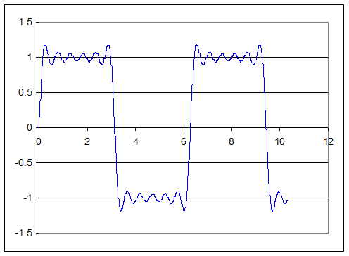
As we include more and more terms, the function becomes smoother but, surprisingly, the initial overshoot at the step stays at a finite fraction of the step height. However, the function recovers more and more rapidly, that is to say, the overshoot and “ringing” at the step take up less and less space. This overshoot is called Gibbs’ phenomenon, and only occurs in functions with discontinuities.

How the Sum over N Terms is Related to the Complete Function

To get a clearer idea of how a Fourier series converges to the function it represents, it is useful to stop the series at $N$ terms and examine how that sum, which we denote $f_{N} (θ)$ , tends towards $f (θ)$ .

So, substituting the values of the coefficients

$\begin{array}{l} A_{n} = \frac{1}{π} \int_{- π}^{π} f (θ) \cos n θ d θ \\ B_{n} = \frac{1}{π} \int_{- π}^{π} f (θ) \sin n θ d θ \end{array}$

in the series

$f (θ) = \frac{A_{0}}{2} + \sum_{n = 1}^{\infty} (A_{n} \cos n θ + B_{n} \sin n θ)$

gives

$\begin{matrix} f_{N} (θ) = \frac{1}{2 π} \int_{- π}^{π} f (θ^{'}) d θ^{'} + \frac{1}{π} \sum_{n = 1}^{N} \int_{- π}^{π} (\cos n θ \cos n θ^{'} + \sin n θ \sin n θ^{'}) f (θ^{'}) d θ^{'} \\ = \frac{1}{2 π} \int_{- π}^{π} f (θ^{'}) d θ^{'} + \frac{1}{π} \sum_{n = 1}^{N} \int_{- π}^{π} \cos n (θ - θ^{'}) f (θ^{'}) d θ^{'} . \end{matrix}$

We can now use the trigonometric identity

$\sum_{n = 1}^{N} \cos n x = \frac{\sin (N + \frac{1}{2}) x}{2 \sin \frac{1}{2} x} - \frac{1}{2}$

to find

$f_{N} (θ) = \frac{1}{2 π} \int_{- π}^{π} \frac{\sin (N + \frac{1}{2}) (θ - θ^{'})}{\sin \frac{1}{2} (θ - θ^{'})} f (θ^{'}) d θ^{'} = \int_{- π}^{π} δ_{N} (θ - θ^{'}) f (θ^{'}) d θ^{'}$

where

$δ_{N} (x) = \frac{1}{2 π} \frac{\sin (N + \frac{1}{2}) x}{\sin \frac{1}{2} x} .$

(Note that proving the trigonometric identity is straightforward: write $z = e^{i x}$ , so $\cos n x = \frac{1}{2} (z^{n} + z^{- n})$ , and sum the geometric progressions.)

Going backwards for a moment and writing

$δ_{N} (x) = \frac{1}{π} (\sum_{n = 1}^{N} \cos n x + \frac{1}{2})$

it is easy to check that

$\int_{- π}^{π} δ_{N} (x) d x = 1.$

To help visualize $δ_{N} (θ)$ , here is $N = 20 :$

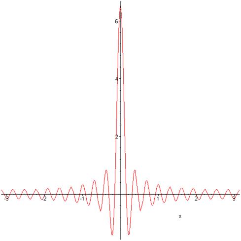
We have just established that the total area under the curve $= 1,$ and it is clear from the diagram that almost all this area is under the central peak, since the areas away from the center are almost equally positive and negative. The width of the central peak is $π / (N + \frac{1}{2})$ , its height $(N + \frac{1}{2}) / π .$

Exercise: for large $N,$ approximately how far down does it dip on the first oscillation? ( $N / π^{2} .$ )

For functions varying slowly compared with the oscillations, the convolution integral

$f_{N} (θ) = \int_{- π}^{π} δ_{N} (θ - θ^{'}) f (θ^{'}) d θ^{'}$

will give $f_{N} (θ)$ close to $f (θ)$ , and for these functions $f_{N} (θ)$ will tend to $f (θ)$ as $N$ increases.

It is also clear why convoluting this curve with a step function gives an overshoot and oscillations. Suppose the function $f (θ)$ is a step, jumping from 0 to 1 at $θ = 0.$ From the convolutionary form of the integral, you should be able to convince yourself that the value of $f_{N} (θ)$ at a point $θ$ is the total area under the curve $δ_{N} (θ)$ to the left of that point (area below zero $—$ that is, below the $x$ -axis $—$ of course counting negative). For $θ = 0,$ this must be exactly 0.5 (since all the area under $δ_{N} (θ)$ adds to 1). But if we want the value of $f_{N} (θ)$ at $θ = π / (2 N + 1)$ (that is, the first point to the right of the origin where the curve cuts through the $x$ -axis), we must add all the area to the left of $θ = π / (2 N + 1)$ , which actually adds up to a total area greater than one, since the leftover area to the right of that point is overall negative. That gives the overshoot.

A Fourier Series in Quantum Mechanics: Electron in a Box

The time-independent Schrödinger wave functions for an electron in a box (here a one-dimensional square well with infinite walls) are just the sine and cosine series determined by the boundary conditions. Therefore, any reasonably smooth initial wavefunction describing the electron can be represented as a Fourier series. The time development can then be found by multiplying each term in the series by the appropriate time-dependent phase factor.

Important Exercise: prove that for a function $f (θ) = \sum_{n = - \infty}^{\infty} a_{n} e^{i n θ}$ , with the $a_{n}$ in general complex,

$\frac{1}{2 π} \int_{- π}^{π} {| f (θ) |}^{2} d θ = \sum_{n = - \infty}^{\infty} {| a_{n} |}^{2} .$

( The physical relevance of this result is as follows: for an electron confined to the circumference of a ring of unit radius, $θ$ is the position of the electron. An orthonormal basis of states of the electron on this ring is the set of functions $(1 / \sqrt{2 π}) e^{i n θ}$ with $n$ an integer, a correctly normalized superposition of these states must have $\sum_{n = - \infty}^{\infty} {| a_{n} |}^{2} = 1$ , so that the total probability of finding the electron in some state is unity. But this must also mean that the total probability of finding the electron anywhere on the ring is unity -- and that’s the left-hand side of the above equation -- the $2 π's$ cancel.)

Exponential Fourier Series

In the previous lecture, we discussed briefly how a Gaussian wave packet in $x$ -space could be represented as a continuous linear superposition of plane waves that turned out to be another Gaussian wave packet, this time in $k$ -space. The plan here is to demonstrate how we can arrive at that representation by carefully taking the limit of the well-defined Fourier series, going from the finite interval $(- π, π)$ to the whole line, and to outline some of the mathematical problems that arise, and how to handle them.

The first step is a trivial one: we need to generalize from real functions to complex functions, to include wave functions having nonvanishing current. A smooth complex function can be written in a Fourier series simply by allowing $A_{n}$ and $B_{n}$ to be complex, but in this case a more natural expansion would be in powers of $e^{i θ}, e^{- i θ} .$

We write:

$f (θ) = \sum_{n = - \infty}^{\infty} a_{n} e^{i n θ} with a_{n} = \frac{1}{2 π} \int_{- π}^{π} e^{- i n θ^{'}} f (θ^{'}) d θ^{'}$

and retracing the above steps

$\begin{matrix} f_{N} (θ) = \frac{1}{2 π} \int_{- π}^{π} \sum_{n = - N}^{N} e^{i n (θ - θ^{'})} f (θ^{'}) d θ^{'} \\ = \frac{1}{2 π} \int_{- π}^{π} f (θ^{'}) d θ^{'} + \frac{1}{π} \int_{- π}^{π} \sum_{n = 1}^{N} \cos n (θ - θ^{'}) f (θ^{'}) d θ^{'} \end{matrix}$ .

exactly the same expression as before, therefore giving the same $δ_{N} (θ)$ . This isn’t surprising, because using $\cos n θ = \frac{1}{2} (e^{i n θ} + e^{- i n θ}), \sin n θ = \frac{1}{2 i} (e^{i n θ} - e^{- i n θ})$ the first $N$ terms in $A_{n}, B_{n}$ can simply be rearranged to a sum over $e^{i n θ}$ terms for $- N \leq n \leq N$ .

Electron out of the Box: the Fourier Transform

To break down a wave packet into its plane wave components, we need to extend the range of integration from the $(- π, π)$ used above to $(- \infty, \infty)$ . We do this by first rescaling from (−π, π ) to (−L/2, L/2) and then taking the limit $L \to \infty .$

Scaling the interval from $2 π$ to $L$ (in the complex representation) gives:

$f (x) = \sum_{n = - \infty}^{\infty} a_{n} e^{2 π i n x / L} where a_{n} = \frac{1}{L} \int_{- L / 2}^{L / 2} f (x) e^{- 2 π i n x / L} d x$

the sum in $n$ being over all integers. This is an expression for $f (x)$ in terms of plane waves $e^{i k x}$ where the allowed $k$ ’s are $2 π n / L$ , with $n = 0, \pm 1, \pm 2, \dots$

Retracing the steps above in the derivation of the function $δ_{N} (x),$ we find the equivalent function to be

$δ_{N}^{L} (x) = \frac{1}{L} (1 + 2 \sum_{n = 1}^{N} \cos \frac{2 π n x}{L}) = \frac{\sin ((2 N + 1) π x / L)}{L \sin (π x / L)} .$

Studying the expression on the right, it is evident that provide $N$ is much greater than $L,$ this has the same peaked-at-the-origin behavior as the $δ_{N} (x)$ we considered earlier. But we are interested in the limit $L \to \infty,$ and there $—$ for fixed N $—$ this function $δ_{N}^{L} (x)$ is low and flat.

Therefore, we must take the limit N going to infinity before taking L going to infinity.

This is what we do in the rest of this section.

Provided $L$ is finite, we still have a Fourier series, representing a function of period $L .$ Our main interest in taking L infinite is that we would like to represent a nonperiodic function, for example a localized wave packet, in terms of plane-wave components.

Suppose we have such a wave packet, say of length $L_{1},$ by which we mean the wave is exactly zero outside a stretch of the axis of length $L_{1} .$ Why not just express it in terms of an infinite $N$ Fourier series based on some large interval $(- L / 2, L / 2)$ provided the wave packet length $L_{1}$ is completely inside this interval? The point is that such an analysis would indeed accurately reproduce the wave packet inside the interval, but the same sum of plane waves evaluated over all the $x$ -axis would reveal an infinite string of identical wave packets $L$ apart! This is not what we want.

As a preliminary to taking L to infinity, let us write the exponential plane wave terms in the standard k-notation,

$e^{2 π i n x / L} = e^{i k_{n} x} .$

So we are summing over an (infinite $N$ ) set of plane waves having wave number values

$k_{n} = 2 π n / L, n = 0, \pm 1, \pm 2, \dots$ ,

a set of equally-spaced $k$ ’s with separation $Δ k = 2 π / L .$

Consider now what would happen if we double the basic interval from $(- L / 2, L / 2)$ to $(- L, L) .$

The new allowed $k$ values are $k_{n} = π n / L, n = 0, \pm 1, \pm 2, \dots$ , so the separation is now $Δ k = π / L,$ half of what it was before. It is evident that as we increase $L,$ the spacing between successive $k_{n}$ values gets less and less.

Going back to the interval of length $L,$ writing $L a_{n} = a (k_{n}), k_{n} = 2 π n / L$ we have

$f (x) = \sum_{n = - \infty}^{\infty} a_{n} e^{2 π i n x / L} = \frac{1}{L} \sum_{n = - \infty}^{\infty} a (k_{n}) e^{i k_{n} x} .$

Recall that the Riemann integral can be defined by

$\int f (k) d k = \lim_{Δ k \to o} \sum f (k_{n}) Δ k$

with $k_{n} = n Δ k, n = 0, \pm 1, \pm 2, \dots$ .

The expression on the right-hand side of the equation for $f (x)$ has the same form as the right-hand side of the Riemann integral definition, and here $Δ k = 2 π / L .$

That is to say,

$\begin{matrix} 2 π f (x) = \frac{2 π}{L} \sum_{n = - \infty}^{\infty} a (k_{n}) e^{i k_{n} x} \\ = \sum_{n = - \infty}^{\infty} a (k_{n}) e^{i k_{n} x} Δ k = \int_{- \infty}^{\infty} a (k) e^{i k x} d k \end{matrix}$

in the limit $Δ k \to 0,$ or equivalently $L \to \infty .$ We are of course assuming here that the function $a (k_{n})$ , which we have only defined (for a given $L$ ) on the set of points $k_{n},$ tends to a continuous function $a (k)$ in the limit $L \to \infty$ .

It follows that in the infinite $L$ limit, we have the Fourier transform equations:

$\begin{matrix} f (x) = \frac{1}{2 π} \int_{- \infty}^{\infty} a (k) e^{i k x} d k and a (k) = \lim_{L \to \infty} L a_{n} \\ = \lim_{L \to \infty} \int_{- L / 2}^{L / 2} f (x) e^{- 2 π i n x / L} d x = \int_{- \infty}^{\infty} f (x) e^{- i k x} d x . \end{matrix}$

Dirac’s Delta Function

Now we have taken both $N$ and $L$ to infinity, what has happened to our function $δ_{N}^{L} (x)$ ? Remember that our procedure for finding $f_{N} (θ)$ in terms of $f (θ)$ gave the equation

$f_{N} (θ) = \frac{1}{2 π} \int_{- π}^{π} f (θ^{'}) d θ^{'} + \frac{1}{π} \int_{- π}^{π} \sum_{n = 1}^{N} \cos n (θ - θ^{'}) f (θ^{'}) d θ^{'}$

Following the same formal procedure with the ( $L = \infty$ ) Fourier transforms, we are forced to take $N$ infinite (recall the procedure only made sense if $N$ was taken to infinity before $L$ ), so in place of an equation for $f_{N} (θ)$ in terms of $f (θ)$ we get an equation for $f (x)$ in terms of itself! Let’s write it down first and think afterwards:

$f (x) = \frac{1}{2 π} \int_{- \infty}^{\infty} (\int_{- \infty}^{\infty} f (x^{'}) e^{- i k x^{'}} d x^{'}) e^{i k x} d k = \int_{- \infty}^{\infty} (\int_{- \infty}^{\infty} \frac{d k}{2 π} e^{i k (x - x^{'})}) f (x^{'}) d x^{'} .$

where

$δ (x) = \int_{- \infty}^{+ \infty} \frac{d k}{2 π} e^{i k x} .$

This is the Dirac delta function. This hand-waving approach has given a result which is not clearly defined. This integral over $x$ is linearly divergent at the origin, and has finite oscillatory behavior everywhere else. To make any progress, we must provide some form of cutoff in $k$ -space, then perhaps we can find a meaningful limit by placing the cutoff further and further away.

From our arguments above, we should be able to recover $δ (x)$ as a limit of $δ_{N}^{L} (x)$ by first taking $N$ to infinity, then $L .$ That is to say,

$δ (x) = \lim_{L \to \infty} (\lim_{N \to \infty} δ_{N}^{L} (x)) = \lim_{L \to \infty} (\lim_{N \to \infty} \frac{\sin ((2 N + 1) π x / L)}{L \sin (π x / L)}) .$

A way to understand this limit is to write $M = (2 N + 1) π / L$ and let $M$ go to infinity before $L .$ (This means as we take $L$ large on its way to infinity, we’re taking $N$ far larger!)

So the numerator is just $\sin M x .$ In the limit of infinite $L,$ for any finite $x$ the denominator is just $π x,$ since $\sin θ = θ$ in the limit of small $θ .$

From this,

$δ (x) = \lim_{M \to \infty} \frac{\sin M x}{π x} .$

This is still a rather pathological function, in that it is oscillating more and more quickly as the infinite limit is taken. This comes about from the abrupt cutoff in the sum at the frequency $N .$

To see how this relates to the (also ill-defined) $δ (x) = \int_{- \infty}^{+ \infty} (d k / 2 π) e^{i k x}$ , recall $δ_{N}^{L} (x)$ came from the series

$δ_{N}^{L} (x) = \frac{\sin (2 N + 1) π x / L}{L \sin π x / L} = \frac{1}{L} (1 + 2 \sum_{n = 1}^{N} \cos \frac{2 π n x}{L}) .$

Expressing the cosine in terms of exponentials, then replacing the sum by an integral in the large $N$ limit, in the same way we did earlier, writing $k_{n} = 2 π n / L$ , so the interval between successive $k_{n}'s$ is $Δ k = 2 π / L,$ so $\int f (k) d k ≅ (2 π / L) \sum f (k_{n}) :$

$δ_{N}^{L} (x) = \frac{1}{L} \sum_{n = - N}^{N} e^{2 π i n x / L} ≅ \int_{- 2 π N / L}^{2 π N / L} \frac{d k}{2 π} e^{i k x} = \frac{\sin (2 π N x / L)}{π x} .$

So it is clear that we’re defining the $δ (x)$ as a limit of the integral $\int_{- 2 π N / L}^{2 π N / L} (d k / 2 π) e^{i k x}$ , which is abruptly cut off at the large values $\pm (2 π N / L) .$ In fact, this is not very physical: a much more realistic scenario for a real wave packet would be a gradual diminution in contributions from high frequency (or short wavelength) modes $—$ that is to say, a gentle cutoff in the integral over $k$ that was used to replace the sum over $n .$ For example, a reasonable cutoff procedure would be to multiply the integrand by $\exp (- Δ^{2} k^{2})$ , then take the limit of small $Δ$ .

Therefore a more reasonable definition of the delta function, from a physicist’s point of view, would be

$\begin{array}{l} δ (x) = \lim_{Δ \to 0} \int_{- \infty}^{+ \infty} \frac{d k}{2 π} e^{i k x} e^{- Δ^{2} k^{2}} \\ = \lim_{Δ \to 0} \frac{1}{{(4 π Δ^{2})}^{1 / 2}} e^{- x^{2} / 4 Δ^{2}} = \lim_{Δ \to 0} δ_{Δ} (x), say . \end{array}$

That is to say, the delta function can be defined as the “narrow limit” of a Gaussian wave packet with total area 1. Unlike the function $δ_{N} (θ)$ , $δ_{Δ} (x)$ has no oscillating sidebands, thanks to our smoothing out of the upper $k$ -space cutoff, so step discontinuities do not generate Gibbs’ phenomenon overshoot -- instead, a step will be smoothed out over a distance of order $Δ$ .

Properties of the Delta Function

It is straightforward to verify the following properties from the definition as a limit of a Gaussian wavepacket:

$\int δ (x) d x = 1, δ (x) = 0 for x \neq 0.$

$δ (x) = δ (- x), δ (a x) = \frac{1}{| a |} δ (x),$

$\int δ (a - x) δ (x - b) d x = δ (a - b) .$

Yet Another Definition, and a Connection with the Principal Value Integral

There is no unique way to define the delta function, and other cutoff procedures can give useful insights. For example, the $k$ -space integral can be split into two and simple exponential cutoffs applied to the two halves, that is, we could take the definition to be

$δ (x) = \lim_{ε \to 0} (\int_{- \infty}^{0} \frac{d k}{2 π} e^{i k x} e^{ε k} + \int_{0}^{+ \infty} \frac{d k}{2 π} e^{i k x} e^{- ε k}) .$

Evaluating the integrals,

$δ (x) = \lim_{ε \to 0} \frac{1}{2 π} (\frac{1}{i x + ε} - \frac{1}{i x - ε}) = \lim_{ε \to 0} \frac{1}{π} (\frac{ε}{x^{2} + ε^{2}}) .$

It is easy to check that this function is correctly normalized by making the change of variable $x = ε \tan θ$ and integrating from $- π / 2 to π /2 .$ This representation of the delta function will prove to be useful later. Note that regarded as a function of a complex variable, the delta function has two poles on the pure imaginary axis at $z = \pm i ε .$

The standard definition of the principal value integral is:

$\int_{- D}^{D} f (x) \frac{P}{x} d x = \lim_{ε \to 0} (\int_{- D}^{- ε} \frac{f (x)}{x} d x + \int_{ε}^{D} \frac{f (x)}{x} d x) .$ this is equivalent to

$\int_{- D}^{D} f (x) \frac{P}{x} d x = \lim_{ε \to 0} \int_{- D}^{D} f (x) \frac{x}{x^{2} + ε^{2}} d x .$

Putting this together with the similar representation of the delta function above, and taking the limit of $ε \to 0$ to be understood, we have the useful result:

$\frac{1}{x \pm i ε} = \frac{P}{x} \mp i π δ (x) .$

Important Exercises:

1. Prove Parseval’s Theorem:

$If f (x) = \int_{- \infty}^{\infty} \frac{d k}{2 π} a (k) e^{i k x}, then \int_{- \infty}^{\infty} {| f (x) |}^{2} d x = \int_{- \infty}^{\infty} \frac{d k}{2 π} {| a (k) |}^{2} .$

2. Prove the rule for the Fourier Transform of a convolution of two functions:

$\begin{array}{l} If f (x) = \int_{- \infty}^{\infty} \frac{d k}{2 π} a (k) e^{i k x}, g (x) = \int_{- \infty}^{\infty} \frac{d k^{'}}{2 π} b (k^{'}) e^{i k^{'} x}, \\ then \int_{- \infty}^{\infty} f (x - x^{'}) g (x^{'}) d x^{'} = \int_{- \infty}^{\infty} \frac{d k}{2 π} a (k) b (k) e^{i k x} . \end{array}$

previous index next PDF