previous index next PDF

Orbital Angular Momentum in Three Dimensions

Michael Fowler 11/05/07

The Angular Momentum Operators in Spherical Polar Coordinates

The angular momentum operator .

In spherical polar coordinates,

the gradient operator is

where now the little hats denote unit vectors: is radially outwards, points along a line of longitude away from the north pole (and therefore in the direction of increasing ) and points along a line of latitude in an anticlockwise direction as seen looking down on the north pole (that is, in the direction of increasing ).

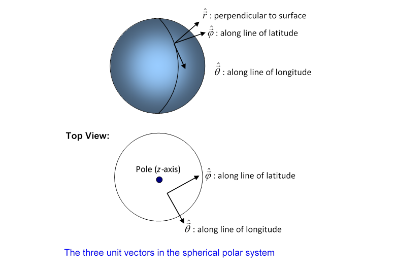
Here form an orthonormal local basis, and

,

as should be clear from the diagram.

So

.

(Explicitly, and .)

The vector has zero component in the z-direction, the vector has component in the z-direction, so we can immediately conclude that

just as in the two-dimensional case.

The operator

To evaluate this expression, we use but we must also check the effects of the differential operators in the first expression on the variables in the second, including the unit vectors.

From the explicit coordinate expressions for the unit vectors, or by staring at the diagram, you should be able to establish the following: is in the r-direction, is a horizontal unit vector pointing inwards perpendicular to , and having component in the -direction, .

Therefore, the only “differentiation of a unit vector” term that contributes to L² is . The acting on the in contributes nothing because .

Hence

Now, we know that L² and L_z have a common set of eigenkets (since they commute) and we’ve already established that those of L_z are , with m an integer, so the eigenkets of L² must have this same f dependence, so they must be of the form , where is a (suitably normalized) solution of the equation

more conveniently written

To summarize: the solutions to this differential equation, with integer will (together with ) give the complete set of eigenstates of L², L_z in the coordinate representation.

Finding the m = l Eigenket of L², L_z

Recall now that for the simple harmonic oscillator, the easiest wave function to find was that of the ground state, the solution of the simple linear equation (as well as being a solution of the quadratic Schrödinger equation, of course). The other state wave functions could then be found by applying the creation operator in differential form the necessary number of times.

A similar strategy works here: we can easily find the highest state on the l ladder, m = l, the state , since it satisfies the linear equation . We just need to cast this equation in coordinate form. In Cartesian coordinates,, and we’ve already shown that .

Therefore

,

and using , we see that , the component of in the + direction, is , and similarly .

So

and becomes

.

That is,

The solution to this equation is

where N is the normalization constant. The wave functions are generated by applying the lowering operator L_- .

Normalizing the m = l Eigenket

The standard notation for the normalized eigenkets is . These functions, being eigenkets of Hermitian operators with different eigenvalues, must satisfy

So, our first job is to normalize (taking already normalized)

The integral can be evaluated using the substitution to give , then making the further substitution to give , which can be integrated by parts to give

.

Therefore

where we have fixed the sign in accord with the standard convention, and we will denote the rather cumbersome normalization constant by c_l.

Notice that for large values of l, this function is heavily weighted around the equator, as we would expect—for a given total angular momentum one gets a maximum component in the z-direction when the motion is concentrated in the x, y plane. This looks like a Bohr orbit.

Finding the Rest of the Eigenkets: the Details

Now that is normalized, we can automatically produce correctly normalized ’s, since we know the matrix element of the lowering operator between normalized states. We don’t have to do any more integrals.

For example, , equivalently (the ’s of course cancel)

That is,

(both terms giving equal contributions).

Note that this function is actually zero on the equator, but for large l it peaks close to the equator (on both sides).

In principle, we can reapply this differential operator over and over to generate all the states, but this gets very messy. However, there is a neat theorem concerning the lowering operator that makes it all straightforward:

Exercise: prove this.

So

and applying the operator again,

So the point of introducing this odd-looking representation of the lowering operator is that the term in the middle is exactly canceled when the operator is applies twice, and similar cancellations occur on repeating the operation, giving the (relatively) simple representation:

(Where did all those factorials come from? They’re the product of all the inverse square root factors in for the number of lowerings necessary.)

Note that for m = 0 the function is

and in fact not a function of at all. This isn’t surprising, since it has zero angular momentum about the z-direction, the appropriate is just constant.

For the differentiation becomes trivial, because, writing , the differentiation becomes and only the term survives, giving

.

Of course, this could also have been found from the linear equation , and we could have equally generated all the states by applying L₊ to this state. In fact, this gives a different—but of course equivalent—expression for the :

(from Messiah, page 522).

Relating the Y_l ^m’s to the Legendre Functions

The Legendre polynomials are defined by:

.

where , so . From this form, it is easy to show that (all n differentiations must take out a factor to give a nonzero contribution), and must have n zeros in the interval (-1, 1). alternates between an even function and an odd function.

The normalization of the ’s is

where in that last line we used the result for the integral obtained earlier in this lecture for normalizing

Doing the same repeated integration by parts for two different Legendre polynomials proves they are orthogonal,

.

The associated Legendre functions are defined (for n and m zero or positive integers, ) by:

Following Messiah in requiring be real and positive, we find

where the coefficient just reflects the differing normalization conventions. Similarly, the spherical harmonics with nonzero m are proportional to the associated Legendre functions (the odd ones are not polynomials in , despite Shankar p. 337, since they include odd powers of ),

The Spherical Harmonics as a Basis

We have found explicit expressions for the spherical harmonics: an orthonormal set of eigenfunctions of L² and L_z defined on the surface of a sphere,

They form a complete set:

or

in the notation of Messiah, where W refers to a point on the spherical surface.

(Formal proof of the completeness is given in Byron and Fuller, Mathematics of Classical and Quantum Physics.)

The above equation could also be written

where the ket is to be understood as a localized ket, the spherical-surface version of , normalized by its d-function inner product with the bra , exactly analogous to , bearing in mind that the infinitesimal area element is , (a positive quantity in the relevant interval, 0 to).

This completeness means that any reasonable function on the surface of the sphere can be expressed as a sum over spherical harmonics with appropriate coefficients, in other words the spherical generalization of a Fourier series.

In fact, L² is equivalent to on the spherical surface, so the are the eigenfunctions of the operator . Just as in one dimension the eigenfunctions of have the spatial dependence of the eigenmodes of a vibrating string, the spherical harmonics have the spatial dependence of the eigenmodes of a vibrating spherical balloon. Of course, to describe the displacement of the balloon skin (which must be real!) with these eigenfunctions, we can no longer use the eigenfunctions of the z-component of angular momentum, since they are complex except in the trivial zero case. We must rearrange the eigenfunctions of L², for example replacing the pair with . These real solutions, essentially , have l nodal lines (zeroes) of longitude. Moving down one notch in , the (real) state with has longitudinal nodes, but has added a latitudinal node: the equator. Then has longitudinal nodes, 2 latitudinal nodal lines—there are always l nodal lines total.

Some of these modes of vibration have been observed in the sun after a sunspot storm. The spherical harmonics are also used in analyzing the cosmic background radiation.

Some Low Order Spherical Harmonics

Let’s look in more detail at the lowest order spherical harmonics. For the first few, the normalization of the highest state is pretty easy to do from scratch: factoring out the dependence as before, , and taking the normalized, the normalization for is just , easily accomplished for

All we then need is , , and finally the sign convention that be real and positive.

With a few elementary steps, it can be established that:

It is often useful to write the in terms of Cartesian coordinates,

so

and

The Y₁^m as a Basis of the l = 1 Subspace

The Y₁^m are the l = 1 eigenstates of L² and L_z. But what if we’d chosen to look for the common eigenstates of L² and L_x instead? What l = 1 state has zero angular momentum component in the direction of the x-axis? Clearly it will be , in other words the previous Y₁⁰ with z replaced by x, because after all, our labeling of axes was arbitrary.

Now,

In fact, any l = 1 state, with a specified component in any direction, can be written as

.

This can be seen as follows: an l = 1 state has to be linear in (any quadratic term would give rise to about an appropriate axis, call that the z-axis, so m = 2 and l must be 2 or greater), and any such state can be written as a linear combination of

.

The bottom line, then, is that the Y₁^m do indeed provide a complete basis for the l = 1 space of eigenstates of L².

Representing the Rotation Operator Within the l = 1 Subspace

Recall that we originally introduced the angular momentum operator by defining it as the generator of infinitesimal rotations when acting on any wave function, including multicomponent wave functions. We found, using the commutativity properties of ordinary rotations, that the vector components of had to satisfy , etc., and from that we deduced the possible sets of eigenvalues of the commuting pair of operators were for , with j an integer of half an odd integer, and for each such j the allowed eigenvalues of were

Back to the l = 1 angular wave functions: we have established that any such function can be written , and so is a vector in a three-dimensional space spanned by the set , In other words, the wave function is a three-component object. The angular momentum operator must therefore be a matrix operator in this three-dimensional space, such that, by definition, the effect of an infinitesimal rotation on the multicomponent wave function is:

The unitary rotation operator acting in the l = 1 subspace, , has to be a matrix. The standard notation for its matrix elements is:

so the rotated ket is

To evaluate this matrix explicitly, we must expand the exponential and we need the matrix elements of between the states —which we already know.

Now, the basis of the three-dimensional space is just the common eigenkets of , in this case identical to . We know the matrix elements of between states from the earlier lecture, so it is simple to find the matrix representations of the components of J in this space:

We have added the superscript (1) because this representation of the infinitesimal rotation operators is specific to j = 1 (representations for general values of j are as matrices, reflecting the dimensionality of the space spanned by the 2j + 1 distinct m values).

Expanding the exponential is not difficult, because by inspection , so from spherical symmetry for a unit vector in any direction. The result is:

One other point we should note: at the end of the linear algebra lecture, we discussed rotations about the z-axis in ordinary (x, y, z) space. Obviously, if we label a point in the (x, y) plane using the complex number x + iy, a rotation by an angle about the z-axis will move the point in such a way that the new label is . The angle in this case has the opposite sign to that given by the operator above: the reason is that when we write the eigenstate as , this is a function of position in the plane, not a point in the plane, so for the reasons discussed at the beginning of the first Angular Momentum lecture, the sign is opposite.

previous index next PDF